Basic Usage

Note

This section is still under development.

Here we introduce the basic usage of BattMo by showing some simple workflows and highlighting important functions.

A First BattMo Model

Let’s make your first BattMo model! 🔋⚡💻

In this example, we will build, run, and visualize a simple P2D simultion for a Li-ion battery cell. We will first introduce how BattMo handles model parameters, then run the simulation, dashboard the results, and explore the details of the simulation output. Finally, we will discuss how to make some basic changes to the model.

Define Parameters

BattMo uses JSON to manage parameters. This allows you to easily save, document, and share complete parameter sets from specific simulations. We have used long and explicit key names for good readability. If you are new to JSON, you can learn more about it here. Details on the BattMo specification are available in the JSON input specification.

For this example, we provide a sample JSON file sample_input.json that describes a simple NMC-Graphite cell.

We load and parse the JSON input file into BattMo using the command:

jsonstruct = parseBattmoJson('Examples/JsonDataFiles/sample_input.json')

This transforms the parameter data as a MATLAB structure jsonstruct that is used to setup the simulation. We can explore the structure within the MATLAB Command Window by navigating the different levels of the structure.

For example, if we want to know the thickness of the negative electrode coating, we can give the command:

jsonstruct.NegativeElectrode.Coating.thickness

which returns:

6.4000e-05

Unless otherwise specified, BattMo uses SI base units for physical quantities.

Run Simulation

We can run the simulation with the command:

output = runBatteryJson(jsonstruct)

Show the Dashboard

We can dashboard the main results using plotDashboard. Here, for example at time step 10,

plotDashboard(output.model, output.states, 'step', 10)

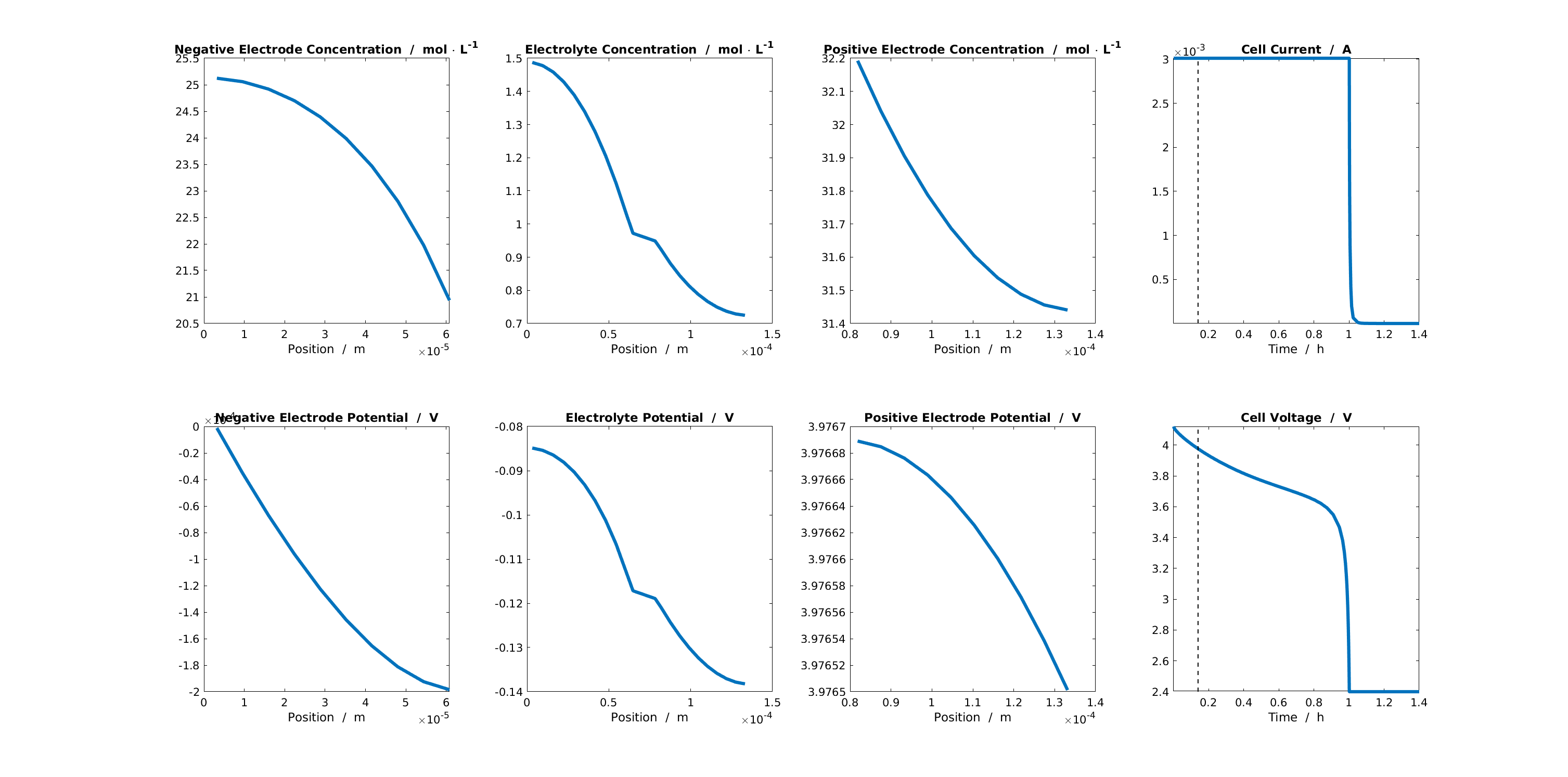
_images/firstresult.png — Dashboard for the solution at a given timestep.

The left 3 columns of the dashboard shows the profiles for the main state quantities (concentration and electric potential) in the negative electrode, electrolyte, and positive electrode. The rightmost column shows the calculated cell current and voltage. In the following subsections, we will explore how to access and plot this data from the simulation output.

Explore the Output

The output structure returns among other thing the model and the states.

model  : [1x1 Battery]
states : [1x1 struct]

The model contains information about the setup of the model and initial conditions, while states contains the results of the simulation at each timestep. Plotting the simulation results requires information about the grid (i.e. what is the position where the quantity is calculated?) and the state (i.e. what is the value of the quantity in that position at a given time?).

Explore the Grid

The grid (or mesh) is one of the most used properties of the model, which can be accessed with the command:

output.model.grid

We can see that the grid is stored as a structure with information about the cells, faces, nodes, etc. The values of the state quantities (e.g. concentration and electric potential) are calculated at the centroids of the cells. To plot the positions of the centroids, we can use the following commands:

x = output.model.grid.cells.centroids;
plot(x, zeros(size(x)), 'o')
xlabel('Position  /  m')

This shows the overall grid that is used for the model. However, BattMo models use a modular hierarchy where the overall cell model is composed of smaller submodels for electrodes, electrolyte, and current collectors. Each of these submodels has its own grid.

For example, if we want to plot the grid associated with the different submodels in different colors, we can use the following commands:

x_ne  = output.model.NegativeElectrode.grid.cells.centroids;
x_sep = output.model.Separator.grid.cells.centroids;
x_pe  = output.model.PositiveElectrode.grid.cells.centroids;

plot(x_ne, zeros(size(x_ne)), 'o')
hold on
plot(x_sep, zeros(size(x_sep)), 'ok')
plot(x_pe, zeros(size(x_pe)), 'or')
xlabel('Position  /  m')

If you would like more information about the BattMo model hierarchy, please see BattMo Model Architecture.

Explore the States

The values of the state quantities at each time step are stored in the states cell array. Each entry in the array describes the state of the simulation at a given timestep.

For example, we can look at the state of the simulation at timestep 10 (shown in the dashboard plot above) using the command:

output.states{10}

which returns the structure:

      Electrolyte: [1×1 struct]
NegativeElectrode: [1×1 struct]
PositiveElectrode: [1×1 struct]
          Control: [1×1 struct]
             time: 504
     ThermalModel: [1×1 struct]

We see that the time of the state is 504 seconds and there are other structures containing the states of the electrodes and electrolyte. We can look into the state of the electrolyte using the command:

output.states{10}.Electrolyte

which shows that there are two quantities there:

  c: [30×1 double]
phi: [30×1 double]

We see that the size of the state quantity vectors match the size of the grid vector.

Plot a Result

Let’s plot the concentration in the electrolyte at timestep 10. We can plot the results using basic MATLAB commands this way:

x = output.model.grid.cells.centroids
c = output.states{10}.Electrolyte.c

plot(x,c)
xlabel('Position  /  m')
ylabel('Concentration  /  mol \cdot m^{-3}')

BattMo also includes dedicated plotting functions that will come in handy when we start working with more complex systems (e.g. P4D grids). We can generate the same plot using the BattMo function plotCellData:

timestep = 10

plotCellData(output.model.grid, output.states{timestep}.Electrolyte.c)
xlabel('Position  /  m')
ylabel('Concentration  /  mol \cdot m^{-3}')

That’s it! 🎉 You have run an post-processed your first simulation! But there are still a lot of exciting features to discover. Let’s keep going and explore making chages to the model. 😃

Change Control Parameters

Let’s try simulating the discharge of the cell at different C-Rates.

Once the JSON parameter file has been read into MATLAB as a jsonstruct, its properties can be modified programmatically. For example, we can define a vector of different C-Rates and then use a for-loop to replace that value in the jsonstruct and re-run the simulation.

CRates = [0.5, 1, 2];
figure()
for i = 1 : numel(CRates)
    jsonstruct.Control.CRate = CRates(i);
    output = runBatteryJson(jsonstruct);

    states = output.states;
    time = cellfun(@(state) state.time, states);
    voltage = cellfun(@(state) state.Control.E, states);
    plot((time/hour), voltage, '-', 'linewidth', 3)
    hold on
end
hold off

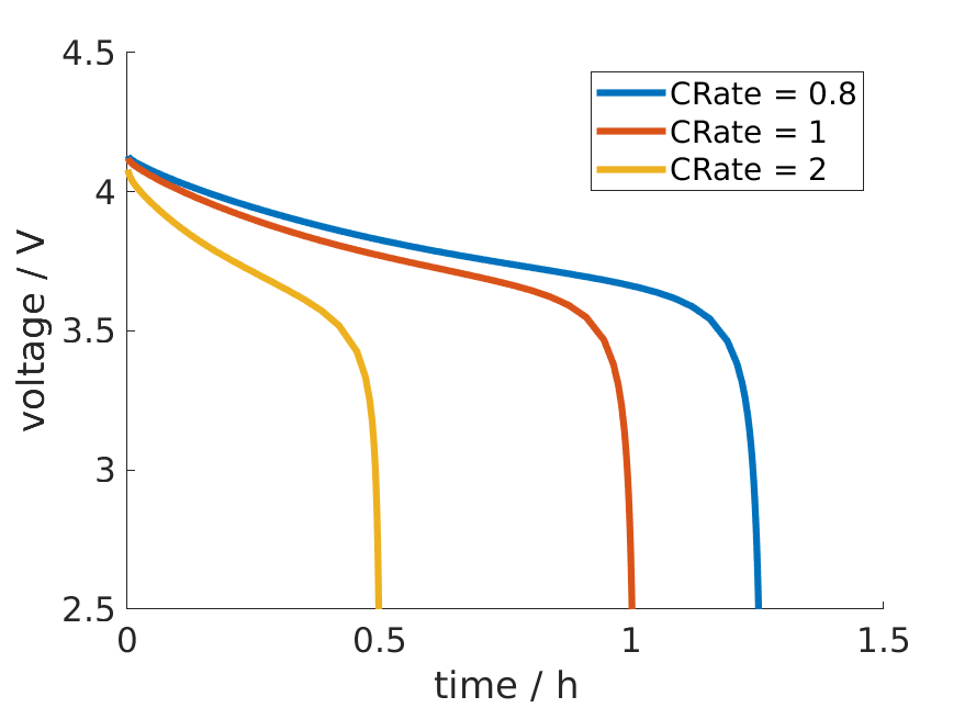
_images/crates.png — A comparison of cell voltage curves at different C-Rates

Change Structural Parameters

Now let’s try changing some structural parameters in the model.

For example, we could simulate the cell considering different thickness values for the negative electrode coating. We will take the same approach as the previous example, by defining a vector of thickness values and using a for-loop to iterate through and re-run the simulation.

thickness = [16, 32, 48, 64].*1e-6;
figure()
for i = 1 : numel(thickness)
    jsonstruct.NegativeElectrode.Coating.thickness = thickness(i);
    output = runBatteryJson(jsonstruct);

    states = output.states;
    time = cellfun(@(state) state.time, states);
    voltage = cellfun(@(state) state.('Control').E, states);
    plot((time/hour), voltage, '-', 'linewidth', 3)
    hold on
end
hold off

From these results we can see that for thin negative electrode coatings, the capacity of the cell is limited by the negative electrode. But the capacity of the negative electrode increases with thickness and eventually the positive electrode becomes limiting.

Change Material Parameters

Finally, let’s try changing active materials in the model.

The sample JSON input file we provided is for an NMC-Graphite cell, but BattMo contains parameter sets for different active materials that have been collected from the scientific literature. Let’s try to replace the NMC active material with LFP.

First, we clear the workspace and reload the original parameter set to start from a clean slate:

clear all
close all
jsonstruct = parseBattmoJson('Examples/JsonDataFiles/sample_input.json');

Now we load and parse the LFP material parameters from the BattMo library and move it to the right place in the model hierarchy:

lfp = parseBattmoJson('ParameterData/MaterialProperties/LFP/LFP.json');
jsonstruct_lfp.PositiveElectrode.Coating.ActiveMaterial.Interface = lfp;

To merge new parameter data into our existing model, we can use the BattMo function mergeJsonStructs.

jsonstruct = mergeJsonStructs({jsonstruct_lfp, ...
                              jsonstruct});

We need to be sure that the parameters are consistent across the hierarchy:

jsonstruct.PositiveElectrode.Coating.ActiveMaterial.density = jsonstruct.PositiveElectrode.Coating.ActiveMaterial.Interface.density;

jsonstruct.PositiveElectrode.Coating.effectiveDensity = 900;

And now, we can run the simulation and plot the discharge curve:

output = runBatteryJson(jsonstruct);

states = output.states;
model  = output.model;

E = cellfun(@(state) state.Control.E, states);
time = cellfun(@(state) state.time, states);

plot(time, E)

Notebooks

We have written and published matlab notebooks in the Live Code File Format (.mlx) .

They basically go through the material described above in the interactive manner.

The notebooks can be found in the Examples/Notebooks directory or downloaded from here.

Tutorial 1	Your first BattMo model	view	download
Tutorial 2	Change the Control Protocol	view	download
Tutorial 3	Modify Structural Parameters	view	download
Tutorial 4	Modify Material Parameters	view	download
Tutorial 5	Simulate CC-CV cycling	view	download
Tutorial 6	Simulate Thermal Performance	view	download
Tutorial 7	A Simple P4D Simulation	view	download
Tutorial 8	Simulate a Multi-Layer Pouch cell	view	download
Tutorial 9	Simulate a Cylindrical Cell	view	download

Next Steps

Congratulations! 🎉 You are now familiar with the BattMo basics!

This should be enough to allow you to setup and run some basic Li-ion battery simulations using P2D grids. Do you want to do more? The Advanced Usage section gives information about setting up custom parameter sets, running simulations in P3D and P4D grids, and including thermal effects.