Protonic Membrane model

Generated from runProtonicMembrane.m

Model overview

We consider the model of a mixed proton and electron conducting membrane, as described in [VST+19] from 2019.

Governing equations

In the membrane, we have three components or species given by the proton (\(H^+\)), and the \(p\) and \(n\) type charge carriers. We need expressions for the fluxes for each of those. The governing equations will then be given by charge and mass conservation equations.

We denote by \(\phi\) the electrostatic potential. For each of the components \(\alpha=\{H^+, p, n\}\), we introduce the electrochemical potential denoted \(\bar\mu_\alpha\) and the chemical potential denoted \(\mu_\alpha\). The potentials are related with each other through the relation

\[\bar\mu_\alpha = \mu_\alpha + z_\alpha F \phi.\]

The fluxes are governed by the gradient of the electrochemical potential. We have

\[j_{\alpha} = -k_\alpha\nabla\bar\mu_\alpha,\]

for some coefficient \(k_\alpha\) which is not necessarily a constant.

We assume that the chemical potential of \(H^+\), that is \(\mu_{H^+}\), is constant in the electrolyte and that \(k_{H^+}\) is constant. Hence, the current density of \(H^+\) is given

\[i_{H^+} = -\sigma_{H^+} \nabla \phi,\]

for a constant conductivity \(\sigma_{H^+}\). We denote by \(E = -\frac{\mu_n}{F}\) the electronic chemical potential and \(\pi = E + \phi\) the electromotive potential. Since we have equilibrium for the n-p reaction, we have the identity

\[d\mu_p + d\mu_n = 0.\]

For the \(p\) and \(n\) type conductivities, we use the empirical relations

\[\sigma_p(E) = \sigma_p^0\exp\left(\frac{F(E - E_{\text{ref},p})}{RT}\right)\quad\text{ and }\quad\sigma_n(E) = \sigma_n^0\exp\left(\frac{-F(E - E_{\text{ref},n})}{RT}\right).\]

Here \(E_{\text{ref},p}\) and \(E_{\text{ref},n}\) are two reference potentials.

We consider the steady state. We could introduce later charge and mass capacitors. The unknowns are the functions \(\phi(x)\) and \(E(x)\) in the electrolyte. The governing equations are given by the mass conservation for the proton and the charge conservation.

The mass conservation equation for \(H^+\) is given by

\[\nabla\cdot j_{H^+} = 0.\]

The total current density is given by \(i = F (j_{H^+} + j_p - j_n)\) and the charge conservation equation is

\[\nabla\cdot i = 0.\]

We introduce the electronic current density \(i_{\text{el}} = F(j_p - j_n)\) and we get

\[\nabla\cdot i_{\text{el}} = 0.\]

We can rewrite \(i_{\text{el}}\) as

\[i_{\text{el}} = - (\sigma_p(E) + \sigma_n(E))\nabla ( E + \phi ).\]

We finally obtain the governing equations for \(\phi(x)\) and \(\pi(x)\) as the following system of differential equations

\[\begin{split}\begin{align} -\nabla\cdot(\sigma_{H^+}\nabla\phi) &= 0,\\ -\nabla\cdot((\sigma_p(E) + \sigma_n(E))\nabla \pi) &= 0. \end{align}\end{split}\]

Boundary conditions

We define the over-potential \(\eta\) as

\[\eta_\text{elde} = \pi_\text{elde} - \phi_\text{elde} - \text{OCP}_\text{elde}\]

where \(\text{OCP}_\text{elde}\) is the open-circuit potential for the given electrode. The value of the OCP at each electrode depend on the composition at the electrode (see [VST+19] for the expressions).

At the anode, we imposte that the proton current is given through the following Buttler-Volmer type expression

\[i_{H^+, \text{an}} = -i_0\frac{e^{-\beta\frac{ z F \eta_{\text{an}}}{RT}} - e^{( 1- \beta)\frac{ z F \eta_{\text{an}}}{RT}}}{ 1+ \frac{i_0}{i_{l,c}}e^{-\beta\frac{ z F \eta_{\text{an}}}{RT}} - \frac{i_0}{i_{l,a}}e^{( 1- \beta)\frac{ z F \eta_{\text{an}}}{RT}}}\]

Here, \(i_{l,c}\) and \(i_{l,a}\) are given constants. The value of the reference current density \(i_0\) is also constant.

The total current is given by \(i_{\text{an}} = I\) for some constant current \(I\).

At the cathode, we impose that the electrostatic potential is equal to zero and a relation between the \(H^+\) current and the over-potential that takes a linear form,

\[R_\text{CT} \ i_{H^+, \text{ct}} = \eta_\text{ct},\]

for a given charge transfer constant \(R_\text{CT}\).

Load and parse input from given json files

The source of the json files can be seen in protonicMembrane.json and 1d-PM-geometry.json

filename = fullfile(battmoDir(), 'ProtonicMembrane', 'jsonfiles', 'protonicMembrane.json');
jsonstruct_material = parseBattmoJson(filename);

filename = fullfile(battmoDir(), 'ProtonicMembrane', 'jsonfiles', '1d-PM-geometry.json');
jsonstruct_geometry = parseBattmoJson(filename);

jsonstruct = mergeJsonStructs({jsonstruct_material, jsonstruct_geometry});

Input structure setup

We setup the input parameter structure which will we be used to instantiate the model

inputparams = ProtonicMembraneInputParams(jsonstruct);

We setup the grid, which is done by calling the function setupProtonicMembraneGrid

[inputparams, gen] = setupProtonicMembraneGrid(inputparams, jsonstruct);

Model setup

We instantiate the model for the protonic membrane cell

model = ProtonicMembrane(inputparams);

The model is equipped for simulation using the following command (this step may become unnecessary in future versions)

model = model.setupForSimulation();

Initial state setup

We setup the initial state using a default setup included in the model

state0 = model.setupInitialState();

Schedule

We setup the schedule, which means the timesteps and also the control we want to use. In this case we use current control and the current equal to zero (see here). We compute the steady-state solution and the time stepping here does not correspond to time values but should be seen as step-wise increase of the effect of the non-linearity (in particular in the expression of the conductivity which includes highly nonlineaer effect with the exponential terms. We do not detail here the method).

schedule = model.Control.setupSchedule(jsonstruct);

Simulation

We run the simulation

[~, states, report] = simulateScheduleAD(state0, model, schedule);

Plotting

We setup som shortcuts for convenience and introduce plotting options

an    = 'Anode';
ct    = 'Cathode';
elyte = 'Electrolyte';
ctrl  = 'Control';

set(0, 'defaultlinelinewidth', 3);
set(0, 'defaultaxesfontsize', 15);

We recover the position of the mesh cell of the discretization grid. This is used when plotting the spatial distribution of some of the variables.

xc = model.(elyte).grid.cells.centroids(:, 1);

We consider the solution obtained at the last time step, which corresponds to the solution at steady-state. The second line adds to the state variable all the variables that are derived from our primary unknowns.

state = states{end};
state = model.addVariables(state, schedule.control);

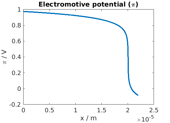
Plot of electromotive potential

figure
plot(xc, state.(elyte).pi)
title('Electromotive potential (\pi)')
xlabel('x / m')
ylabel('\pi / V')

Plot of electronic chemical potential

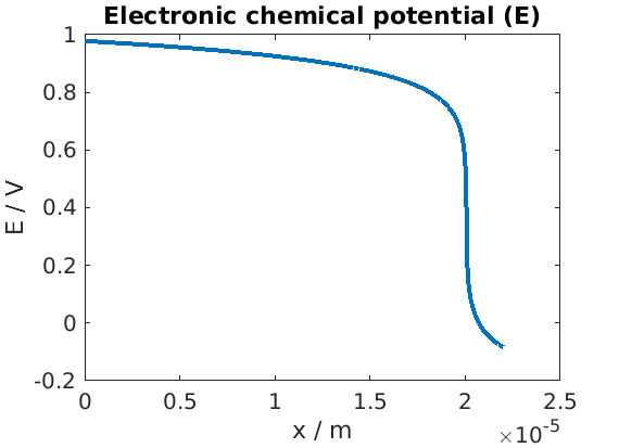
figure
plot(xc, state.(elyte).pi - state.(elyte).phi)
title('Electronic chemical potential (E)')
xlabel('x / m')
ylabel('E / V')

Plot of electrostatic potential

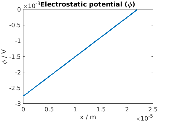
figure
plot(xc, state.(elyte).phi)
title('Electrostatic potential (\phi)')
xlabel('x / m')
ylabel('\phi / V')

Plot of the conductivity

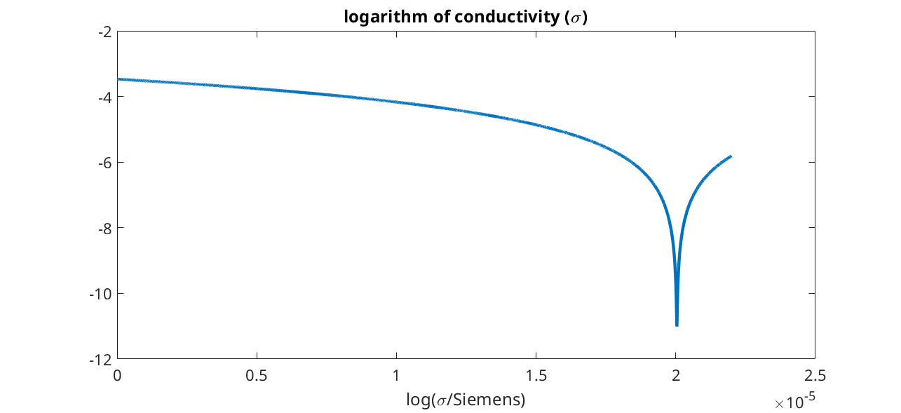
figure
plot(xc, log(state.(elyte).sigmaEl))
title('logarithm of conductivity (\sigma)')
xlabel('x / m')
xlabel('log(\sigma/Siemens)')

Evolution of the Faradic efficiency

We increase the current density from 0 to 1 A/cm^2 and plot the faraday efficiency. We sample the current value from 0 to 1 A/cm^2.

Is = linspace(0, 1*ampere/((centi*meter)^2), 20);

We run the simulation for each current value and collect the results in the endstates.

endstates = {};
for iI = 1 : numel(Is)

    model.Control.I = Is(iI);
    [~, states, report] = simulateScheduleAD(state0, model, schedule);

    state = states{end};
    state = model.addVariables(state, schedule.control);

    endstates{iI} = state;

end

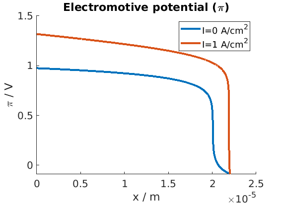
We plot the profile of the electromotive potential for the mininum and maximum current values.

figure
hold on

unit = ampere/((centi*meter)^2); % shortcut

state = endstates{1};
plot(xc, state.(elyte).pi, 'displayname', sprintf('I=%g A/cm^2', Is(1)/unit));
state = endstates{end};
plot(xc, state.(elyte).pi, 'displayname', sprintf('I=%g A/cm^2', Is(end)/unit));

title('Electromotive potential (\pi)')
xlabel('x / m')
ylabel('\pi / V')
legend

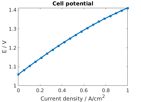
We retrieve and plot the cell potential

E = cellfun(@(state) state.(an).pi - state.(ct).pi, endstates);

figure
plot(Is/unit, E, '*-');
xlabel('Current density / A/cm^2')
ylabel('E / V')
title('Cell potential');

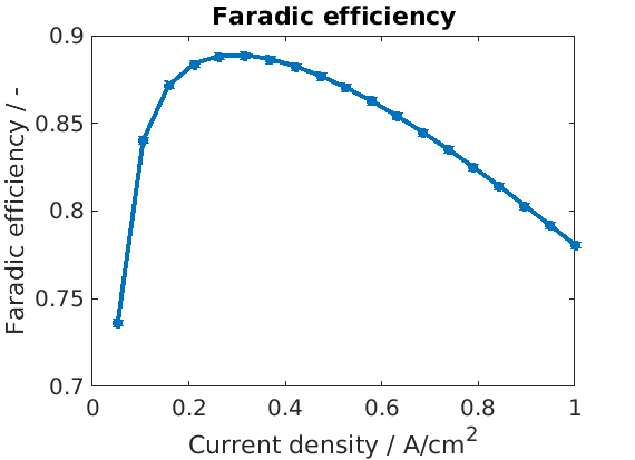
We retrieve and plot the Faradic efficiency

feff = cellfun(@(state) state.(an).iHp/state.(an).i, endstates);

figure
plot(Is/unit, feff, '*-');
xlabel('Current density / A/cm^2')
ylabel('Faradic efficiency / -')
title('Faradic efficiency');

complete source code can be found here