Computation Graph Model Design ang Assembly

Introduction

We consider a generic physical system for which a mathematical model has been proposed. The mathematical model introduces variables and equations. Some of the variables are state variables in the sense that they directly fully describe the state of system. We call those variables primary variables. Other variables are defined through explicit dependencies from the primary variables. We call those variables secondary variables. The equations are then formulated as functions of the primary and/or secondary variables whose values should be equal to zero. As such, an equation, or more precisely the left-hand side of it, is a secondary variable, the right-hand side of the equatio being zero. We call the left-hand side of an equation, its residuals.

In the setting we are interested in, that is numerical simulation, the primary variables are the unknown which we want to compute by solving the equations. For many system, some of the state variables are functions of time and/or space. The corresponding equations take then the form of ordinary and/or partial differential equations. A first task of the solver is then to discretize the variables and setup a system of equations in finite dimension. We assume here that this step is done and we will look at the variables as vector variables.

primary variables	unknown	\(x_1,...,x_n\)
secondary variables	explicit expressions \(y_i(x_1, ..., x_n)\)	\(y_1,...,y_p\)
equations	\(f_i(x_1, ..., x_n, y_1, ..., y_p)= 0\)	residuals \(f_1, ..., f_q\)

A mathematical model introduces a set of variables and of functional relationships between the variables. Typically, the variables introduced in the model have a specific name which reflects their physical significance. We want to preserve the terminology introduced by the model as it is essential for its understanding. We recognize then the structure of a directed graph, where the nodes corresponds the variable names and the edges connect the variable through the functional dependencies introduced by the model.

In the example below, we have 3 primary variables, 2 secondary and 3 equations. A model gives us definitions of the secondary variables and the equations, for example,

\[\begin{split}y_1 &= y_1(x_1, x_2, y_2) \\ y_2 &= y_1(x_1, x_2, x_3)\\\end{split}\]

with the equations

\[\begin{split}f_1(y_1, y_2) &= 0\\ f_2(y_1, y_2, x_2) &= 0\\ f_3(x_1, x_3) &= 0\end{split}\]

This information is completly contained in the following graph

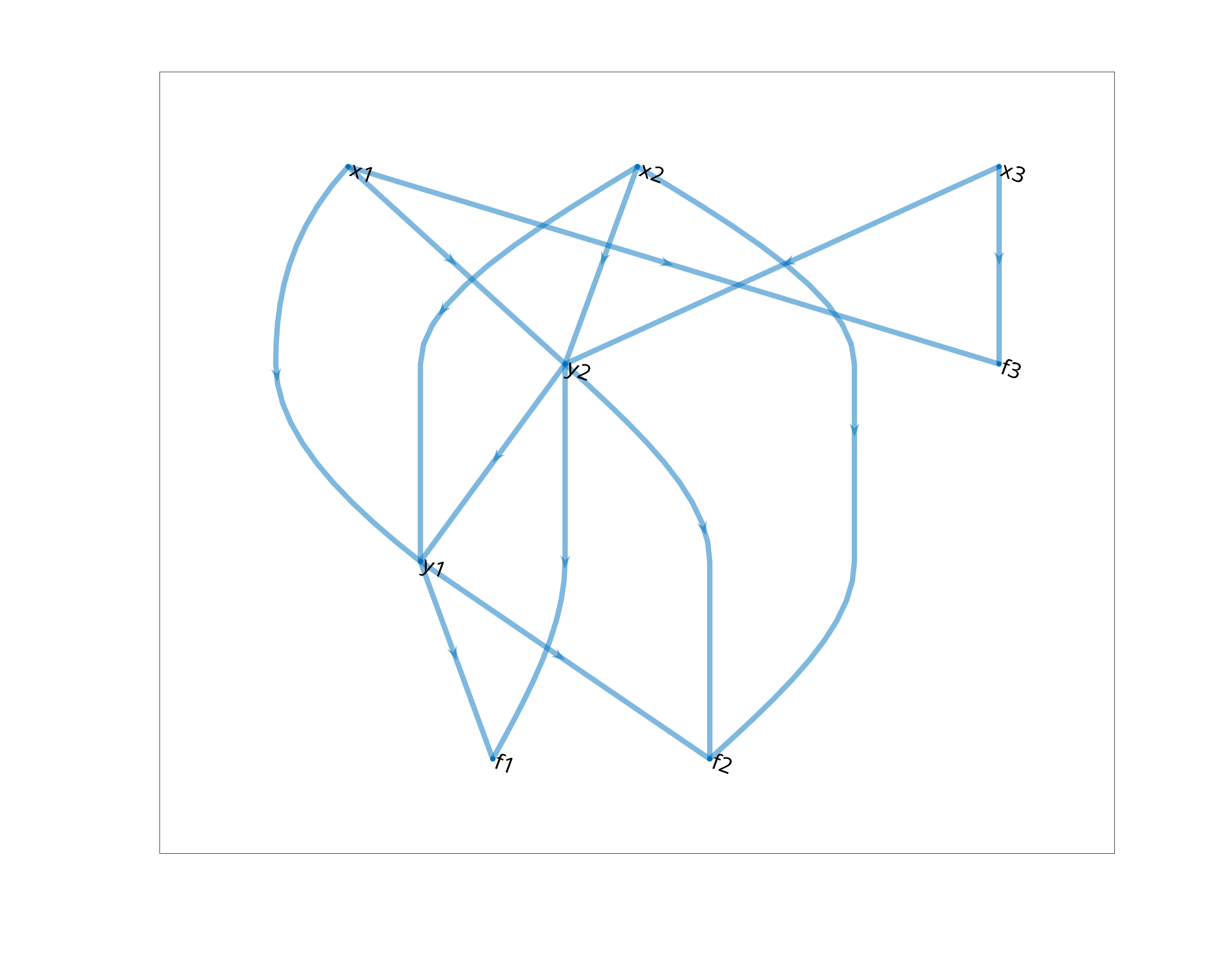
Given a mathematical model, we can therefore create a computational graph by collecting the variable names and encoding the variable dependencies in edges, as the one presented above.

We observe that a computational graph offers a very usefull synthetic overview of a model. This observation will be hopefully confirmed by the example below.

Model assembly

When solving a system of equation, an important task for the solver is the assembly of the equations: Given the values of the primary variables, \(x_i\), we want to compute the values of the residuals, \(f_i\).

To do so we have to evaluate the intermediate secondary variables. The evaluation of the secondary variables up to the residuals can only be done in an order that is compatible with the functional dependencies.

A compatible order can be obtained from the computational graph by using a topological sorting.

The order of the update sequence is not unique. For the example above, a possible sequence is to update

\[y_2, f_3, y_1, f_2 \text{, and finally } f_1\]

It is usefull to have a solver where the decleration of the computational graph can be done before implementing the update functions. In this way, we break the complexity in the implementation of a model. The first step is the design of the graphs, which can be done using interactive tools (see below), where we also declare all the update functions. Those are however implemented in a second step. Then, we can focus on them at the apriopriate scope level (see model hierarchy) not distracted by the overall architecture. The solver can then automatically generate from the sequence of function calls that will be used to update all the residuals.

By using computational graph we aim at improving:

1. model explorability

2. model reusability using model hierarchy and composition

Model explorability

We consider a user that is given a simulation code which corresponds to a given physical system. The user may want to understand the mathematical model which is implemented in this simulator. All the variable definitions are of course implemented in the code but they are not easily accessible. We can use a computational graph interactively to get an overview of all the variables that are computed and, given a variable, be sent to the place in the code where the variable is computed. There, the user finds the precise definition.

As we will see, models are implemented in a hierarchy. This structure contributes also to an easier model exploration. The variable dependency is declared at the lowest level in the model hierarchy so that, isolated from the rest, it is easier to understand.

Model hierarchy and composition

As model developper, we want to reuse as much as possible existing models.

Model explorability is important to inspect the already available models, understand their structure and figure out how they can be modified to our need.

The computational graph provides a very synthetic representation on the model an in a first step, the model developper should only focus on getting the computational graph that corresponds to his/her model.

In the code of a given, there is a method where the computational graph is defined, see the example below. The developper gets there the possibility to edit the computational graph. The actions available are

1. Add new variables to the model (meaning adding nodes to the computational graph).

2. Add functional dependencies (meaning adding directed edges from the function input variables nodes to the function output variable node).

3. Change the declared functional dependencies.

4. Change the status of the variables (see static variables below)

A simple and concrete way to create a new model from a given one is to setup a derived model using class inheritance. The new model will inherit the computational graph, which is a property of the model. We will see an example below.

Models are often obtained by coupling physical sub-systems. Each of the sub-systems are models in themselves. For us, it means that they have a computational graph. Coupling models will then consist of

1. Importing the graphs of the subsystems

2. Adding functional dependencies across the sub-models (adding edges that connect the nodes of the graphs)

We can see this operation as sewing graphs. Concretely, we proceed by creating a new model and register the models we want to couple as sub-models. Each sub-model should be given a name. The graphs of all sub-models are imported and the names of the variables (the nodes) are extended with a kind of prefix which corresponds to the sub-model it originates from. This action is necessary to avoid name conflicts. Indeed, the sub-models have been developed independently and nothing guarantees that they do not share some of the same variable names.

By repeatedly coupling models, we obtain a hierarchy of models. A model can get very complex but having a hierarchy significantly simplifies the navigation between the sub-models and the understanding of how they depend on each other.

When a computational graph is setup or modified, we do not say anything about the function that will in practice update the variables - besides their name. We do not need a computational graph framework to develop models but we need precise definitions of the functions the defines the variables.

Basic Example

by existing models, and reuse the variable update functions that are been defined there. Looking at the graph, we can understand the dependency easily and identify the part that should be changed in the model. In some cases, the dependency graph may not changed, only a different function should be called to update a variable. For example, the exchange current density function \(j\) rarely obeys the ideal case presented above but is a given tabulated function,

\[j(c_e, c_s) = \hat{j}(c_s, c_s)\]

where \(\hat{j}\) is a given function the user has set up. Such function is an example of a functional parameter belonging to the model, which we mentioned earlier.

Continuing with the same example, we may introduce a temperature dependency in the OCP function. We have

\[\text{OCP} = \hat{\text{OCP}}(c_s, T)\]

Then, we have to introduce a new node (i.e. variable) in our graph, the temperature T.

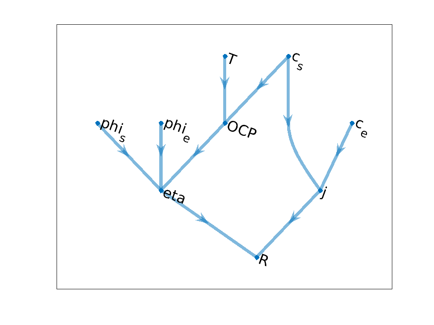
Reaction model graph with added temperature

Let us introduce an other model, at least its computational graph. We consider a simple heat equation

\[\alpha T_t = \nabla\cdot(\lambda \nabla T) + q\]

We introduce in addition to the temperature T the following variable names (nodes) and, in the right column, we write the definition they will take after discretization. The operators div and grad denotes the discrete differential operators used in the assembly.

accumTerm	\(\alpha\frac{T - T^0}{\Delta t}\)
flux	\(-\lambda\text{grad}(T)\)
sourceTerm	\(q\)
energyCons	\(\text{accumTerm} + \text{div}(\text{flux}) + \text{source}\)

The computational for the temperature model is given by

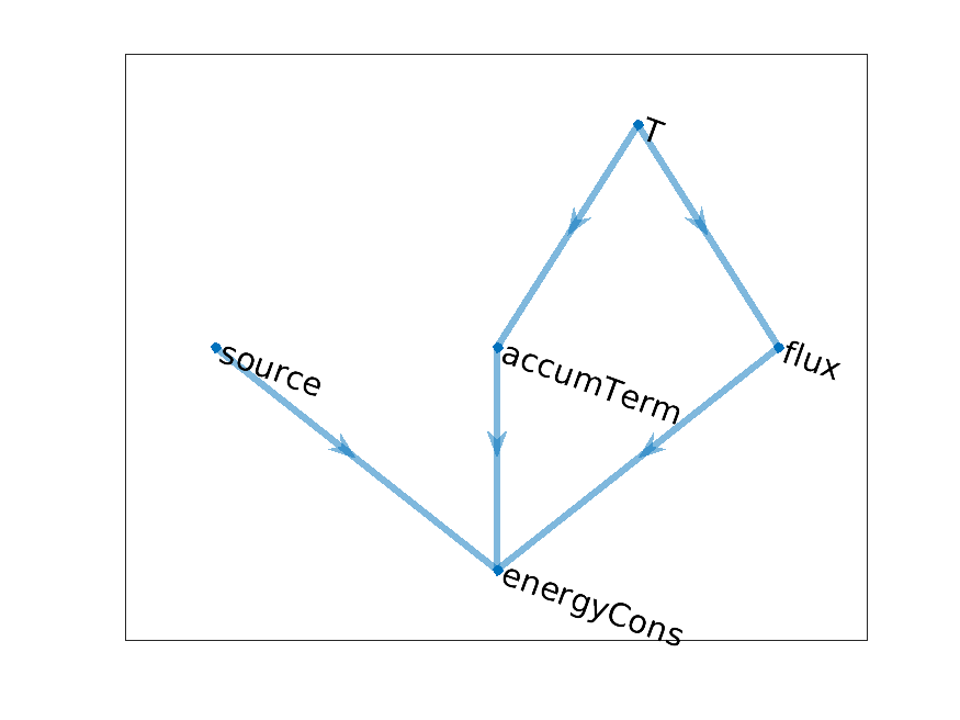
Temperature model graph

Having now two models, we can illustrate how we can combine the corresponding computational graph to obtain a coupled model. Let us couple the two models in two ways. We include a heat source produced by the chemical reaction, as some function of the reaction rate. The effect of the temperature on the chemical reaction is included, as we presented earlier, as a additional temperature dependence of the open circuit potential OCP. We obtain the following computational graph

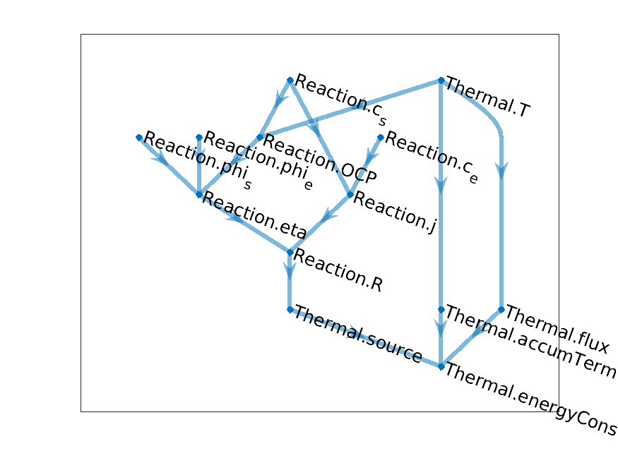
Coupled Temperature Reaction model graph

In the node names, we recognize the origin of variable through a model name, either Reaction or Thermal. We will come back later to that.

With this model, we can setup our first simulation. Given the concentrations and potentials, we want to obtain the temperature, which can only obtained implicitely by solving the energy equation. Looking at the graph, we find that the root variables are Thermal.T, Reaction.c_s, Reaction.phi_s, Reaction.c_e, Reaction.phi_e. The tail variable is the energy conservation equation energyCons. A priori, the system looks well-posed with same number of unknown and equation (one of each). At this stage, we want our implementation to automatically detects the primary variables (the root node, T) and the equations (the tail node, energyCons) and to proceed with the assembly by traversing the graph. We will later how it is done.

To conclude this example, we introduce a model for the concentrations and make them time dependent. In the earlier model, the concentrations were kept constant because, for example, access to an infinite reservoir of the chemical species. Now, we consider the case of a closed reservoir and the composition evolve accordingly to the chemical reaction. We have equations of the form

\[\begin{align*} \frac{dc_s}{dt} &= R_s, & \frac{dc_r}{dt} &= R_e \end{align*}\]

where the right-hand side is obtained from the computed reaction rate, following the stoichiometry of the chemical reactions.

The computational grap for each of this equation take the generic form

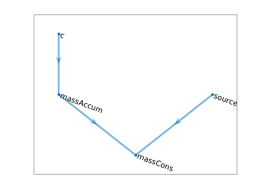
Concentration model graph

where

masssAccum	\(\frac{c - c^0}{\Delta t}\)
source	\(R\)
massCons	\(\frac{c - c^0}{\Delta t} - R\)

Let us now combine this model with the first one, which provided us with te computation of the chemical reaction rate. We need two instance of the concentration model. To solve, the issue of duplicated variable name, we add indices in our notations but this cannot be robustly scaled to large model. Instead, we introduce model names and a model hierarchy. This was done already earlier with the Thermal and Reaction models. Let us name our two concentration models as Solid and Elyte. We obtain the following graph.

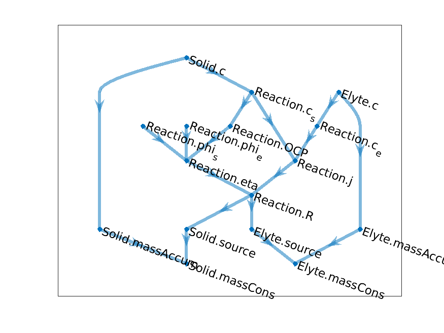
Coupled reaction-concentration model

We note that it becomes already difficult to read off the graph and it will become harder and harder as model grow. We have developped visualization tool that will help us in exploring the model through their graphs.

Given phi_s and phi_e, we can solve the problem of computing the evolution of the concentrations. The root nodes are the two concentrations (the potentials are known) and the tail nodes are the mass conservation equations.

Finally, we can couple the model above with with the temperature, by sewing together the graphs. We name the previous composite model as Masses and keep the name of Thermal for the thermal model. We obtain the following

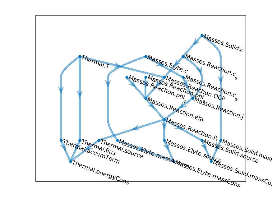
Coupled Temperature-Concentration-Reaction graph

New computational graphs are thus obtained by connecting existing graph, using a hierarchy of model. In the example above, the model hierarchy is given by

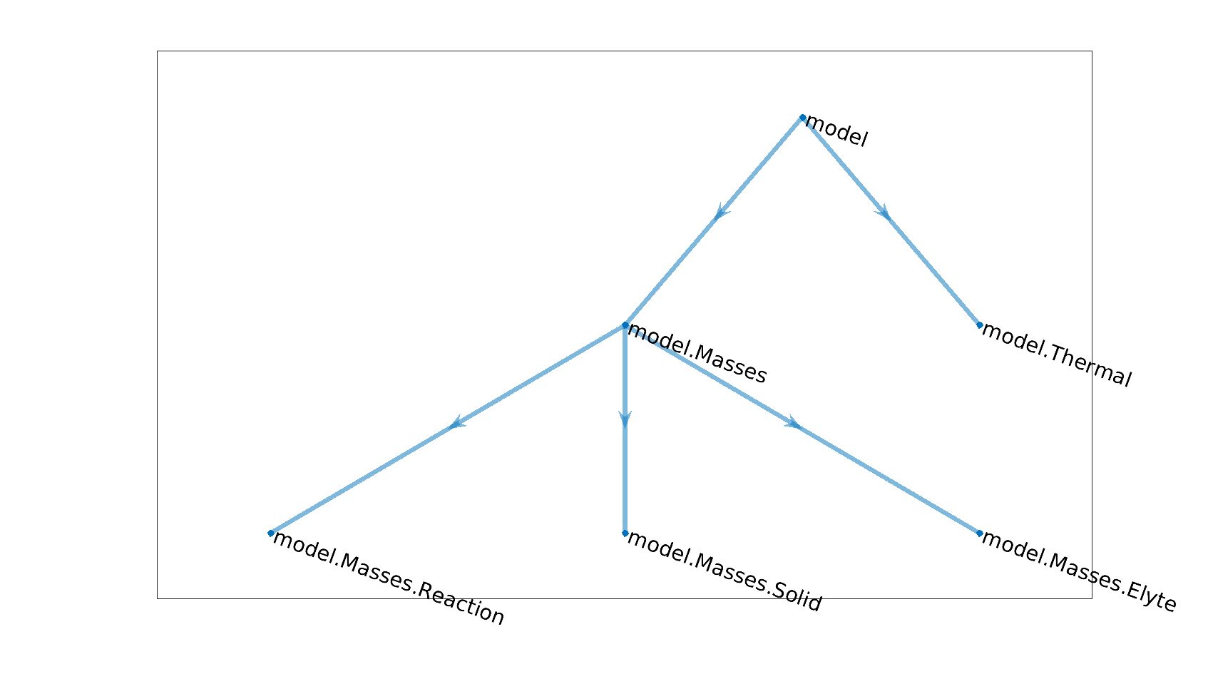
Model hierarchy

The graph of a parent model is essentially composed of the graphs of its child models with the addition of a few new edges which connect the graphs of the child models. The graph of the parent model can also bring its own new variables.

Graph Setup and Implementation

The implementation of a model can be decomposed into two steps.

1. We setup the computational graph.

2. We implement the functions corresponding to each node with incoming edges.

Our claim is that this decomposition breaks the complexity in the implementation of large coupled models. Once the two steps above are done, a Newton loop in our simulator will consist of

1. Instantiation of the primary variables (the root nodes) as AD (Automatic Differentiation) variables

2. Evaluation of all the functions in a order that can be infered by the graph, as it gives us the relative dependencie between all the variables

3. Assembly of the Jacobian obtained form the residual equations (the tail nodes)

The Jacobian matrix with the residuals can be sent to a Newton solver which will return an update of the primary variables, until convergence. All these three steps can by automatised as we will see later, so that a user which wants to implement a new model can only focus on the two steps mentioned further up.

We need now to provide the user with a framework for computational graph and functionalities to setup graphs easily within this framework. Let review the functionalities we want to include.

The overall goals are readibility and reusabililty. For code reusability, we want to be able to reuse in an easy way any function that have been implemented in existing models. For the graph framework it implies that graphs can always be modified at any level. A modification of an existing model consists of changing its graph and add or replace functions that have to be changed or replace but keeping all the other functions unchanged. We should be able to setup our assembly step 2 using these functions untouched. We will see how we solve this requirement.

A graph, in general, is determined by the nodes and edges. Typically a graph description is done by indexing the nodes and edges are described by a pair of node index. In our case, the indexing is done internally in processing of the model. At the setup level for the user, we want to use variable names (string) because they are supposed to have a meaning for the user and a model designer is going to choose those carefully in order to enhance the readibility of its model. When, we combine graphs we face the issue of shared names by the two graphs. Since the models have been likely implemented independently, we have to deal with this issue. We solve it by using a name space mechanism. For a given variable name, indices are frequently needed and should be supported. A typical example is a chemical system which brings different species, each of them bringing a concencentration variable. To get a generic implementation, it is impractical to deal with the names of each of the species and we rather use indices, over which it is easy to iterate. A map between species name in index can be conveniently introduced. We end up with the following structure for a variable name, a class called VarName see VarName with the following properties

classdef VarName

  properties

     namespace % Cell array of strings
     name      % String
     dim       % Integer
     index     % Array of integer or string ':'

  end

Within a model (i.e. a graph) all the variables (i.e. nodes) have a unique name. A new model can be created by combining existing models. Each of those should be assigned a unique name, which we be added to the name space. We end up with a graph of unique names. The process is the same as module import in programming language such as Python or Julia.

We can use the example above to illustrate the mechanism. At the three different model levels (reaction model, coupled reaction-concentration model and coupled temperature-reaction-concentration model), the concentration of the solid electrode takes different names

model	namespace	name
reaction	{}	'c_s'
reaction-concentration	{'Reaction'}	'c_s'
temperature-reaction-concentration	{'Masses', 'Reaction'}	'c_s'

We use two instances of the concentration model in the coupled reaction-concentration model. Namespace is needed to distinguish between those,

namespace	name
{'Solid'}	c
{'Elyte'}	c

Let us introduce the code functionalities for constructing models. For the moment, we focus on the the nodes (variable names). Later, we will look at the edges (functional dependencies). We use the temperature model as an example. The class BaseModel is, at its name indicates, the base class for all models. We will introduce gradually the most usefull methods for this class. For our temperature model, we start with

classdef ThermalModel < BaseModel

    methods

        function model = registerVarAndPropfuncNames(model)

            %% Declaration of the Dynamical Variables and Function of the model
            % (setup of varnameList and propertyFunctionList)

            model = registerVarAndPropfuncNames@BaseModel(model);

            varnames = {};
            % Temperature
            varnames{end + 1} = 'T';
            % Accumulation term
            varnames{end + 1} = 'accumTerm';
            % Flux flux
            varnames{end + 1} = 'flux';
            % Heat source
            varnames{end + 1} = 'source';
            % Energy conservation
            varnames{end + 1} = 'energyCons';

            model = model.registerVarNames(varnames);

        end
    end
end

The most impatient can have a look of the complete implementation of ThermalModel. The method registerVarAndPropfuncNames is used to setup all that deals with the graph in a given model. We called the method registerVarNames to add a list of nodes in our graph given by varnames.

Note

The variable name is given by a single string here and not a instance of VarName. This is a syntaxic sugar and internally the variable name T is converted to VarName({}, 'T', 1, ':')

To lighten the graph setup, we have introduced at several places syntaxic sugar.

We can now instantiate the model, setup the computational graph. The graph is given as a ComputationalGraphInteractiveTool class instance. This class provides some computational and inspection methods that acts on the graph.

model = ThermalModel();
model = model.setupComputationalGraph();
cgt   = model.computationalGraph;

We have written a shortcut for the two last lines

cgt =  model.cgt;

When the computational graph is setup, the property varNameList of BaseModel is populated with VarName variables. We will rarely look at this list directly. Instead, we use the method printVarNames in ComputationalGraphInteractiveTool which, as its name indicates, print the variables that have been registered.

>> cgt.printVarNames()

T
source
accumTerm
flux
energyCons

Similary, we setup a reaction model as follows

classdef ReactionModel < BaseModel

    methods

        function model = registerVarAndPropfuncNames(model)

            model = registerVarAndPropfuncNames@BaseModel(model);

            varnames = {};
            % potential in electrode
            varnames{end + 1} = 'phi_s';
            % charge carrier concentration in electrode - value at surface
            varnames{end + 1} = 'c_s';
            % potential in electrolyte
            varnames{end + 1} = 'phi_e';
            % charge carrier concentration in electrolyte
            varnames{end + 1} = 'c_e';
            % Electrode over potential
            varnames{end + 1} = 'eta';
            % Reaction rate [mol s^-1 m^-2]
            varnames{end + 1} = 'R';
            % OCP [V]
            varnames{end + 1} = 'OCP';
            % Reaction rate coefficient [A m^-2]
            varnames{end + 1} = 'j';

            model = model.registerVarNames(varnames);

        end
    end
end

(For the impatient, the full implementation which includes the properties is available here). As expected, we obtain the following output

>> model = ReactionModel();
>> cgt = model.cgt;
>> cgt.printVarNames

phi_s
c_s
phi_e
c_e
OCP
j
eta
R

Let us now couple the two models. We introduce a new model which has in its properties an instance of the ReactionModel and of the ThermalModel. The name of the properties is use to determine the namespace. We write

classdef ReactionThermalModel < BaseModel

    properties

        Reaction
        Thermal

    end

    methods

        function model = ReactionThermalModel()

            model.Reaction = ReactionModel();
            model.Thermal  = ThermalModel();

        end

    end

end

We can already instantiate this model (for the impatient, the full model setup is available here).

>> model = ReactionThermalModel();
>> cgt = model.cgt;
>> cgt.printVarNames();

Reaction.phi_s
Reaction.c_s
Reaction.phi_e
Reaction.c_e
Thermal.T
Reaction.OCP
Reaction.j
Thermal.accumTerm
Thermal.flux
Reaction.eta
Reaction.R
Thermal.source
Thermal.energyCons

We now observe how the new model has all the variables from both the sub models and they have been assigned a namespace which prevents ambiguities. In the printed form above, the name space components are joined with a dot delimiter and added in front of the name. The VarName variable that corresponds to the first name in the printed list above is VarName({'Reaction'}, 'phi_s')

Let us now look at how we declare the edges, with corresponds for us to the function that update some of the variables. For some of the variables, we declare the fact that the variable will be updated by calling a function where the arguments are given by other variables (i.e. nodes) given in the graph. In this way we obtain directed edges. The class to encode this information is PropFunction. The properties for the class are the following

classdef PropFunction

    properties

        varname             % variable name that will be updated by this function

        inputvarnames       % list of the variable names that are arguments of the function

        modelnamespace      % model name space

        fn                  % function handler for the function to be called

        functionCallSetupFn % function handler to setup the function call

    end

A PropFunction tells us that the variable with name varname will be updated by the function fn which will only require in its evaluation the value of the variables contained in the list inputvarnames. In addition, we have the name space of a model where the parameters to evaluate the function can be found. Earlier, we explained that most functions need external parameters to be evaluated and those are stored in the properties of some model. The location of this model is given by modelnamespace. The function is going to called automatically in the assembly process (step 2). The property functionCallSetupFn is used to setup this call. Let us now look at the complete listing of the thermal model

classdef ThermalModel < BaseModel

    methods

        function model = registerVarAndPropfuncNames(model)
            
            model = registerVarAndPropfuncNames@BaseModel(model);
            
            varnames = {};
            % Temperature
            varnames{end + 1} = 'T';
            % Accumulation term
            varnames{end + 1} = 'accumTerm';
            % Flux flux
            varnames{end + 1} = 'flux';
            % Heat source
            varnames{end + 1} = 'source';
            % Energy conservation
            varnames{end + 1} = 'energyCons';
            
            model = model.registerVarNames(varnames);
            
            fn = @ThermalModel.updateFlux;
            model = model.registerPropFunction({'flux', fn, {'T'}});

            fn = @ThermalModel.updateAccumTerm;
            model = model.registerPropFunction({'accumTerm', fn, {'T'}});
            
            fn = @ThermalModel.updateEnergyCons;
            inputnames = {'accumTerm', 'flux', 'source'};            
            model = model.registerPropFunction({'energyCons', fn, inputnames});

            
        end

    end
    
end

We have declared three property function using the method registerPropFunction

Note

The method registerPropFunction offers syntaxic sugar, which is very important to keep the implementation concise. If we did not use any syntaxic sugar, the declaration of the flux property function would be as follows

fn            = @ThermalModel.updateFlux;
inputvarnames = {VarName({}, 'T')};
varnname      = VarName({}, 'flux');

propfunction = PropFunction(varname, fn, inputvarnames, {});

model = model.registerPropFunction(propfunction);

We can instantiate this model and use the ComputationalGraphPlot tool to visualize the resulting graph.

model = ThermalModel();
cgp = model.cgp(); % "cgp" stands for "computational graph plot"
cgp.plot();

We obtain the plot we already presented above

Temperature model graph

We can use the printOrderedFunctionCallList method of the ComputationalGraphInteractiveTool class to print the sequence of function calls that is used to update all the variables in the model ThermalModel, which examplify how we can automatize the assembly. The order of the function evaluation is computed from the graph structure.

>> cgt = model.cgt
>> cgt.printOrderedFunctionCallList

Function call list
state = model.updateAccumTerm(state);
state = model.updateFlux(state);
state = model.updateEnergyCons(state);

Similarly we implement the property functions of the reaction model, see here. The corresponding graph is plotted above

For the sake of the illustration we introduce and UncoupledReactionThermalModel, which consists only of the following line (see also here)

classdef UncoupledReactionThermalModel < BaseModel
    properties
        Reaction
        Thermal
    end
    methods
        function model = UncoupledReactionThermalModel()
            model.Reaction = ReactionModel();
            model.Thermal  = ThermalModel();
        end
    end
end

We can instantiate the model and plot the graph

model = UncoupledReactionThermalModel
cgp = model.cgp
cgp.plot

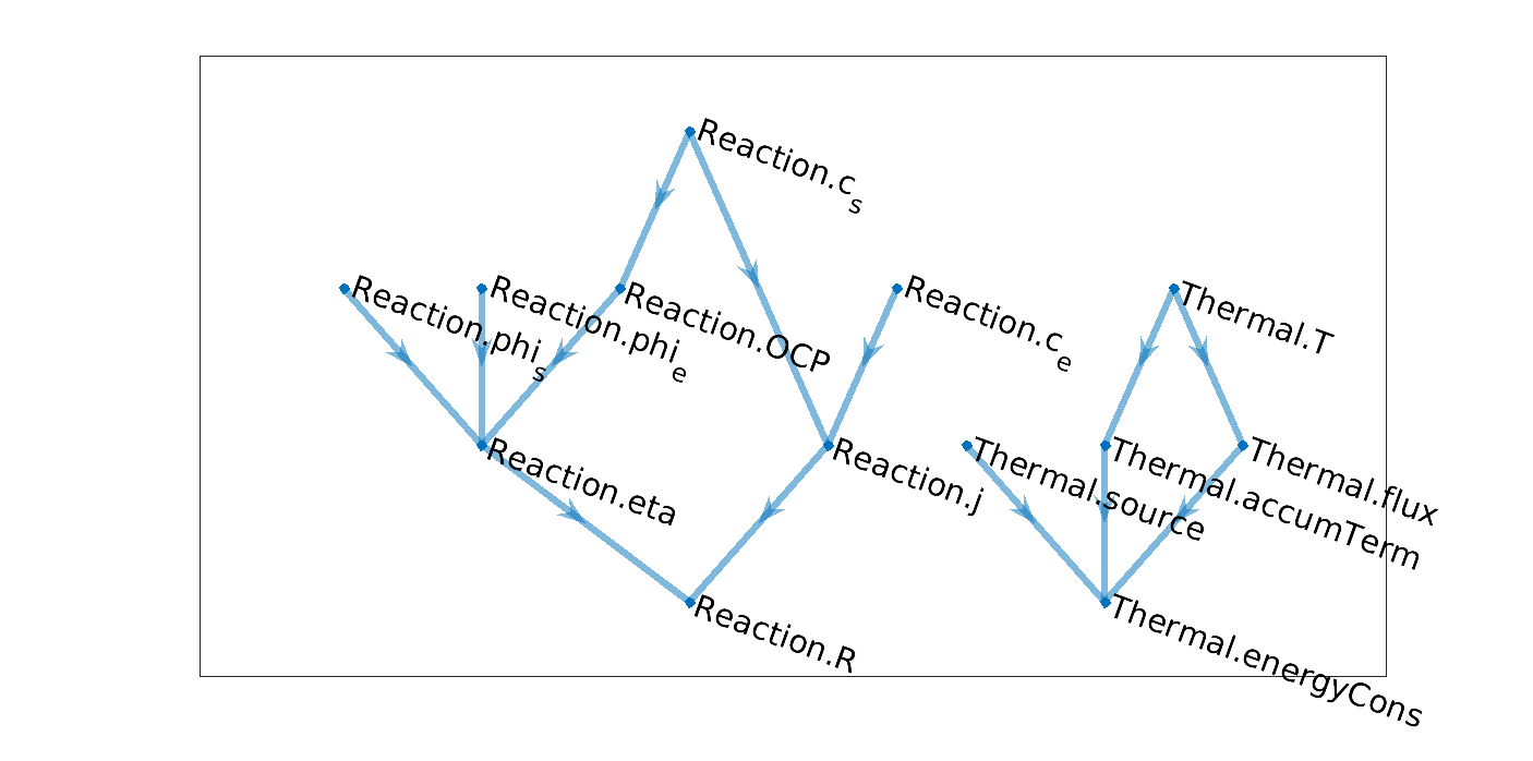
Uncoupled thermal reaction model.

The variable name and graph structures are imported from both the submodels. The name of the model it originates from is added to the name of each variable. We can clearly see that the two graphs of the sub-models are uncoupled as no edge connect them to each other.

We implement the coupling between the models, as announced here, using the following setup (see also here), which coupled the OCP to the temperature and the source term of the energy equation to the reaction rate.

classdef ReactionThermalModel < BaseModel

    properties

        Reaction
        Thermal
        
    end
    
    methods

        function model = ReactionThermalModel()

            model.Reaction = ReactionModel();
            model.Thermal  = ThermalModel();
            
        end
        function model = registerVarAndPropfuncNames(model)
            
            %% Declaration of the Dynamical Variables and Function of the model

            model = registerVarAndPropfuncNames@BaseModel(model);

            fn = @ReactionThermalModel.updateOCP;
            inputnames = {{'Reaction', 'c_s'}, {'Thermal', 'T'}};
            model = model.registerPropFunction({{'Reaction', 'OCP'}, fn, inputnames});

            fn = @ReactionThermalModel.updateThermalSource;
            inputnames = {{'Reaction', 'R'}};
            model = model.registerPropFunction({{'Thermal', 'source'}, fn, inputnames});
            
        end

    end
    
end

In this case, we obtain the following list of function calls

>> model = ReactionThermalModel();
>> cgt = model.cgt;
>> cgt.printOrderedFunctionCallList;

Function call list
state = model.updateOCP(state);
state.Reaction = model.Reaction.updateReactionRateCoefficient(state.Reaction);
state.Thermal = model.Thermal.updateAccumTerm(state.Thermal);
state.Thermal = model.Thermal.updateFlux(state.Thermal);
state.Reaction = model.Reaction.updateEta(state.Reaction);
state.Reaction = model.Reaction.updateReactionRate(state.Reaction);
state = model.updateThermalSource(state);
state.Thermal = model.Thermal.updateEnergyCons(state.Thermal);

From this example, we can understand how we can fullfill the requirement we set above, where we formulate the goal that we want to call a function without have to modify it at all, whereever in the model hierarchy the variable that will be updated belongs to. For that, we use simple matlab structure mechanism. Here, we sse that the values of the thermal variables (T, flux, …) are stored in the Thermal field of the state variable, so that when we send the variable state.Thermal to the function updateFlux (for example), the variables coming from the other submodel Reaction are stripped off. The function updateFlux implemented in the ThermalModel will only see a state variable with the fields it knows about, locally, at the level of the model.