Optimization
The topic of optimization does not only involve finding the parameters that maximizes some output quantity such as the energy output. Optimization, from a mathematical viewpoint, also involve fitting parameters in the numerical model against data, for example provided by experiments. This procedure has many names, including “fitting”, “parameterization”, “calibration” and “parameter identification”. We will here present an example of parameter identification followed by an example of optimization.
Parameter identification example
The complete source code of this example can be found at runParameterIdentification.
As often, we start by defining our MRST modules and some convenient short names. In particular, we instantiate the optimization module, which provides the key classes and functions for performing optimization.
mrstModule add ad-core optimization mpfa mrst-gui

clear
close all

ne      = 'NegativeElectrode';
pe      = 'PositiveElectrode';
elyte   = 'Electrolyte';
thermal = 'ThermalModel';
am      = 'ActiveMaterial';
co      = 'Coating';
itf     = 'Interface';
sd      = 'SolidDiffusion';
ctrl    = 'Control';
sep     = 'Separator';
Then we set up the battery: the chemistry, the geometry, how it is operated (the control) and the time stepping, as discussed in the other tutorials. Here, an option for validating the json struct is included but set to false by default since the validation requires MATLAB to call Python, which in turn requires a compatible Python version installed. If you are interested in testing this, set the flag to true.
In addition there is commented code for setting up a finer time discretization. This is because later in the tutorial we will see the effect of using a finer time discretization and stricter tolerances.
jsonParams  = parseBattmoJson(fullfile('ParameterData', 'BatteryCellParameters', 'LithiumIonBatteryCell', 'lithium_ion_battery_nmc_graphite.json'));
jsonGeom    = parseBattmoJson(fullfile('Examples', 'JsonDataFiles', 'geometry1d.json'));
jsonControl = parseBattmoJson(fullfile('Examples', 'JsonDataFiles', 'cc_discharge_control.json'));
jsonSim     = parseBattmoJson(fullfile('Examples', 'JsonDataFiles', 'simulation_parameters.json'));

json = mergeJsonStructs({jsonParams, jsonGeom, jsonControl, jsonSim});

json.Control.useCVswitch = true;

% % Test finer time discretization
% json.TimeStepping.numberOfTimeSteps = 80;
% json.TimeStepping.numberOfRampupSteps = 10;

% Optionally validate the json struct
validateJson = false;
The json struct completely specifies the simulation. We simulate the model and save the output in a conventient data structure. This will form the initial data for the parameter identification later on.
json0 = json;
output0 = runBatteryJson(json0, 'validateJson', validateJson);

simSetup = struct('model'   , output0.model   , ...
                  'schedule', output0.schedule, ...
                  'state0'  , output0.initstate);
In this example we will fit five parameters:
the Bruggeman coefficient for the electrolyte
the exchange current densities for both electrodes
the volumetric surface areas for both electrodes
To set up these parameters in the fitting, we use the ModelParameter class in MRST. As can be seen in the source code found at ModelParameter, there are a several options that can be set. The most important ones are the ones used here:
the name of the parameter (arbitrary)
the object to which the parameter belongs (usually model)
the boxLims, which sets hard constraints for the range of the parameters
the scaling, which is linear per default, but may be logarithmic
the location of the parameter in the object (model)
params = addParameter(params, simSetup, ...
            'name', 'elyte_bruggeman', ...
            'belongsTo', 'model', ...
            'boxLims', [1, 3], ...
            'location', {elyte, 'bruggemanCoefficient'});

% Exchange current densities in the Butler-Volmer eqn
params = addParameter(params, simSetup, ...
                      'name', 'ne_k0', ...
                      'belongsTo', 'model', ...
                      'scaling', 'log', ...
                      'boxLims', [1e-12, 1e-9], ...
                      'location', {ne, co, am, itf, 'reactionRateConstant'});
params = addParameter(params, simSetup, ...
                      'name', 'pe_k0', ...
                      'belongsTo', 'model', ...
                      'scaling', 'log', ...
                      'boxLims', [1e-12, 1e-9], ...
                      'location', {pe, co, am, itf, 'reactionRateConstant'});

% Volumetric surface areas
params = addParameter(params, simSetup, ...
                      'name', 'ne_vsa', ...
                      'belongsTo', 'model', ...
                      'boxLims', [1e5, 1e7], ...
                      'location', {ne, co, am, itf, 'volumetricSurfaceArea'});
params = addParameter(params, simSetup, ...
                      'name', 'pe_vsa', ...
                      'belongsTo', 'model', ...
                      'boxLims', [1e5, 1e7], ...
                      'location', {pe, co, am, itf, 'volumetricSurfaceArea'});
In the next step we generate what we may call “experimental” data, i.e. data that we will calibrate against (as we will shortly seen, we will use the “experimental” voltage E_exp and current I_exp). This data is generated by running a simulation with average values of the boxLims as values for the parameters in params. This makes the resulting optimization problem very easy to solve, but still illustrates the basic workflow of setting up parameter identification problems.
jsonExp = json;
pExp = zeros(numel(params), 1);
for ip = 1:numel(params)
  loc = params{ip}.location;
  orig = params{ip}.getfun(simSetup.(params{ip}.belongsTo), loc{:});
  new = mean(params{ip}.boxLims);
  jsonExp = params{ip}.setfun(jsonExp, loc{:}, new);
  pExp(ip) = new;
end
outputExp = runBatteryJson(jsonExp, 'validateJson', validateJson);
Next we set up the objective function, i.e. the function we seek to minimize by varying the parameters params. We set this to be a least squares function of the differences of the “experimental” values and the values that will be obtained during the optimization. The least squares function here is formed by both the voltages E and the currents I: obj(E, I) = ||E - E_exp||^2 + ||I - I_exp||^2.
To make sure the objective function is correct, we test it by evaluating it using the generated “experimental” values to make sure it is zero.
Physics-based models are often costly to simulate accurately, because they are often large and nonlinear. Since multiple evaluations of the model must likely be done during optimization, we want an algorithm that is as efficient as possible in the sense that we want to evaluate the model as few times as possible. One approach for accomplishing this is to take information from the gradients into account, so-called gradient-based optimization methods. The function that will compute the gradients of the objective function with respect to params is also set up here. Under the hood, BattMo will compute these by solving the adjoint problem.
% Objective function
objective = @(model, states, schedule, varargin) leastSquaresEI(model, states, outputExp.states, schedule, varargin{:});

% Debug: the objective function evaluated at the experimental values
% should be zero
objval = objective(outputExp.model, outputExp.states, outputExp.schedule);
assert(max(abs([objval{:}])) == 0.0);

% Function for gradient computation
objVals = objective(output0.model, output0.states, output0.schedule);
objScaling = sum([objVals{:}]);
objectiveGradient = @(p) evalObjectiveBattmo(p, objective, simSetup, params, 'objScaling', objScaling);
To make sure the adjoint gradients are correct, we can compare them with gradients calculated by a classical finite difference approximation. The relative difference between them should not be too large, and it can also be useful to simply look at the sign. This is such a basal check that during development, the commented return statement below can be uncommented until the objective function is correctly set up.
debug = true;
if debug
  pTmp = getScaledParameterVector(simSetup, params);

  [vad, gad] = evalObjectiveBattmo(pTmp, objective, simSetup, params, ...
                                   'gradientMethod', 'AdjointAD');

  [vnum, gnum] = evalObjectiveBattmo(pTmp, objective, simSetup, params, ...
                               'gradientMethod', 'PerturbationADNUM', ...
                               'PerturbationSize', 1e-7);
  fprintf('Adjoint and finite difference derivatives and the relative error\n');
  disp([gad, gnum, abs(gad-gnum)./abs(gad)])

  %return
end
Now we are ready to perform the optimization. We use the well-tested, efficient BFGS method with the parameters set by params. The initial guess is deduced from the belongsTo and location properties in the params vector. Note that the parameters are actually scaled to [0, 1] using the boxLims. After the optimization, these will be scaled back.
We may set up several criteria for the BFGS method to terminate:
gradTol: BFGS terminates if the gradient is less than this value.
objChangeTol: BFGS terminates if the change in the objective function is less than this value.
maxIt: BFGS terminates after these many iterations.
Also note that we set maximize=false, since we perform a minimization: we want to minimize the least squares functional.
Note that we have commented out a stricter value for objChangeTol. It is of great interest to see how using this value in combination with the finer temporal discretization will change the result. In fact, numerous numerical properties influence the optimization. Not only the parameters of the BFGS method, but also the space and time discretization parameters and solver tolerances also may play a role.
p0scaled = getScaledParameterVector(simSetup, params);
gradTol = 1e-7;
objChangeTol = 1e-4;
%objChangeTol = 1e-7;
maxIt = 25;
[v, pOptTmp, history] = unitBoxBFGS(p0scaled      , objectiveGradient, ...
                                    'maximize'    , false            , ...
                                    'gradTol'     , gradTol          , ...
                                    'objChangeTol', objChangeTol     , ...
                                    'maxIt'       , maxIt            , ...
                                    'logplot'     , true);
numIt = numel(history.val);
After waiting for BFGS to finish (a couple of minutes on a standard laptop), we run the model with the optimized parameters, optionally plot the result and display the relative difference between the “experimental”, and optimized values.
jsonOpt = json;

for ip = 1:numel(params)
    loc = params{ip}.location;
    jsonOpt = params{ip}.setfun(jsonOpt, loc{:}, pOpt(ip));
end

outputOpt = runBatteryJson(jsonOpt, 'validateJson', validateJson);

%%
do_plot = true;
if do_plot
    set(0, 'defaultlinelinewidth', 2)

    getTime = @(states) cellfun(@(state) state.time, states);
    getE = @(states) cellfun(@(state) state.Control.E, states);

    t0 = getTime(output0.states);
    E0 = getE(output0.states);
    tOpt = getTime(outputOpt.states);
    EOpt = getE(outputOpt.states);
    tExp = getTime(outputExp.states);
    EExp = getE(outputExp.states);

    h = figure; hold on; grid on; axis tight
    plot(t0/hour, E0, 'displayname', 'E_{0}')
    plot(tExp/hour, EExp, '--', 'displayname', 'E_{exp}');
    plot(tOpt/hour, EOpt, ':', 'displayname', 'E_{opt}')
    legend;

end

%% Summarize
pOrig = cellfun(@(p) p.getParameter(simSetup), params)';

fprintf('Initial guess:\n');
fprintf('%g\n', pOrig);

fprintf('Fitted values (* means we hit the box limit):\n');
tol = 1e-3;
for k = 1:numel(params)
    hit = '';
    if abs(pOptTmp(k)) < tol || abs(pOptTmp(k)-1) < tol
        hit = '*';
    end
    fprintf('%g %s\n', pOpt(k), hit);
end

fprintf('\nExperimental values:\n');
fprintf('%g\n', pExp);

fprintf('\nRelative error between optimized and experimental values:\n')
fprintf('%g\n', relErr);

fprintf('\nIterations:\n')
fprintf('%g\n', numIt);
The exact values obtained may depend how default parameters of BattMo are set, but at the time of writing we get
       name               pOpt         pExp
___________________    __________    _________
{'elyte_bruggeman'}        1.6149            2
{'ne_k0'          }    4.2599e-11    5.005e-10
{'pe_k0'          }    1.8927e-11    5.005e-10
{'ne_vsa'         }    2.9014e+05     5.05e+06
{'pe_vsa'         }     4.018e+05     5.05e+06
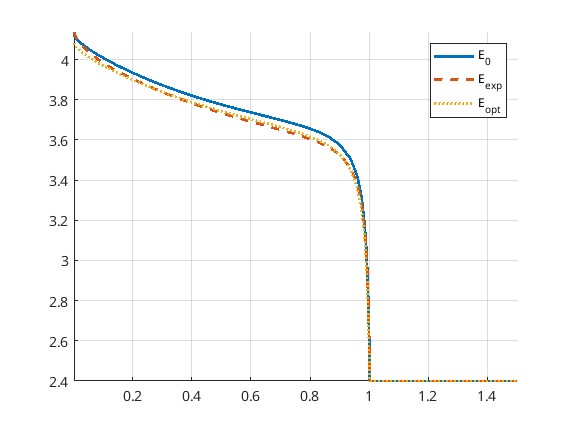
The match of the discharge voltage using the default setup is shown in the figure below. It’s good towards the end, but not so much in the beginning. Here
E_0 is the voltage using the parameters from the initial guess
E_exp is the “experimental” voltage that we seek to match
E_opt is the voltage from the optimized parameters
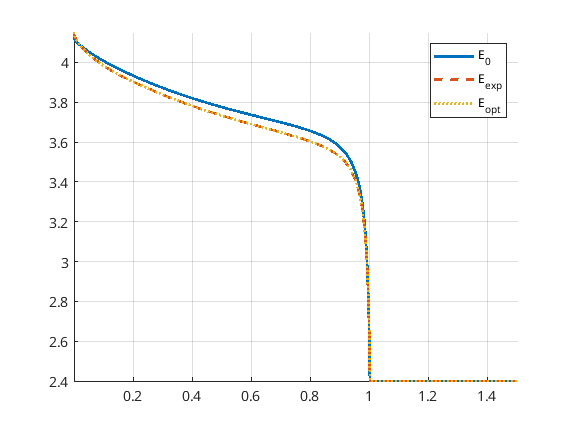
Now we can uncomment the parts of the code that give a finer time discretization and a stricter tolerance for BFGS as discussed above. Running the program again results in a very good match, both in the parameters and the discharge potential curve. Note that we reach the boxLim for ne_k0, why a next step could be to change this.
      name               pOpt         pExp
___________________    __________    _________
{'elyte_bruggeman'}        1.9998            2
{'ne_k0'          }         1e-09    5.005e-10
{'pe_k0'          }    3.4029e-10    5.005e-10
{'ne_vsa'         }    2.4994e+06     5.05e+06
{'pe_vsa'         }    4.7775e+06     5.05e+06
Optimization example
Here we will present an example illustrating how the energy output of a battery in one cycle can maximized by adjusting the porosity and the operating current. The complete code is available at runBattery1DOptimize.
We start by clearing the workspace, closing figures and initializing the MRST modules.
% Clear the workspace and close open figures
clear
close all

% Load MRST modules
mrstModule add ad-core mrst-gui mpfa optimization
For this example we set up a standard Li-ion battery with an NMC cathode and graphite anode without currect collectors. At the moment, we do not take into account thermal effects, and we use a simple diffusion model. This means that the diffusion in the active material is determined by evaluating an analytical function, in contrast to the standard approach, where the diffusion is determined by solving a 1D differential equation. The difference should not be that significant in this case, and the ambitious reader is encouraged to investigate this.
jsonstruct = parseBattmoJson(fullfile('ParameterData','BatteryCellParameters','LithiumIonBatteryCell','lithium_ion_battery_nmc_graphite.json'));
jsonstruct.include_current_collectors = false;
jsonstruct.use_thermal = false;

% We define some shorthand names for simplicity.
ne      = 'NegativeElectrode';
pe      = 'PositiveElectrode';
am      = 'ActiveMaterial';
cc      = 'CurrentCollector';
elyte   = 'Electrolyte';
thermal = 'ThermalModel';
itf     = 'Interface';
sd      = 'SolidDiffusion';
ctrl    = 'Control';
sep     = 'Separator';

jsonstruct.(ne).(am).diffusionModelType = 'simple';
jsonstruct.(pe).(am).diffusionModelType = 'simple';

inputparams = BatteryInputParams(jsonstruct);

inputparams.(ctrl).useCVswitch = true;
To avoid too much computational cost, we set up a P2D model.
gen = BatteryGeneratorP2D();

% Now, we update the inputparams with the properties of the grid.
inputparams = gen.updateBatteryInputParams(inputparams);

%  Initialize the battery model.

model = Battery(inputparams);
To avoid an initial strong shock to the system, we ramp-up the current to the prescribed current using small time steps. An appropriate default control (the procedures for how the battery is to be operated) that does this is set up automatically by the built-in function setupScheduleControl.
% Smaller time steps are used to ramp up the current from zero to its
% operational value. Larger time steps are then used for the normal
% operation.

CRate = model.Control.CRate;
total = 1.2*hour/CRate;

n    = 40;
dt   = total*0.7/n;
step = struct('val', dt*ones(n, 1), 'control', ones(n, 1));

% Setup the control by assigning a source and stop function.

control = model.Control.setupScheduleControl();

nc = 1;
nst = numel(step.control);
ind = floor(((0 : nst - 1)/nst)*nc) + 1;

step.control = ind;
control.Imax = model.Control.Imax;
control = repmat(control, nc, 1);

schedule = struct('control', control, 'step', step);
Then we set up the nonlinear solver. To illustrate the capabilities of the nonlinear solver we lower the default maximum number of iterations and set a tolerance depending on the input current. The solver will cut the time steps in half if the nonlinear system fails to converge, resulting in so-called “ministeps”. When running the simulation, we have the option to return values at these ministeps (see the call to simulateScheduleAD below).
nls = NonLinearSolver();

% Change the number of maximum nonlinear iterations
nls.maxIterations = 10;

% Change default behavior of nonlinear solver, in case of error
nls.errorOnFailure = false;

% Change tolerance for the nonlinear iterations
model.nonlinearTolerance = 1e-3*model.Control.Imax;

% Set verbosity
model.verbose = false;
Given an initial state, we can now solve the system. Note that we pass our nonlinear solver object and set OutputMinisteps=true as options. We may also plot the resulting potential.
% Setup the initial state
initstate = model.setupInitialState();

% Run the simulation
[~, states, ~] = simulateScheduleAD(initstate, model, schedule, 'OutputMinisteps', true, 'NonLinearSolver', nls)

ind = cellfun(@(x) not(isempty(x)), states);
states = states(ind);

E    = cellfun(@(x) x.Control.E, states);
I    = cellfun(@(x) x.Control.I, states);
time = cellfun(@(x) x.time, states);

doPlot = false;

if doPlot
    figure;
    plot(time/hour, E, '*-', 'displayname', 'initial');
    xlabel('time  / h');
    ylabel('voltage  / V');
    grid on
end
The energy of the cell is calculated by calling the EnergyOutput function or simply by evaluating the integral E*I*dt using the trapezoidal rule. The reason for introducing the EnergyOutput function is that this will be used as objective function in the optimization below.
obj = @(model, states, schedule, varargin) EnergyOutput(model, states, schedule, varargin{:});
vals = obj(model, states, schedule);
totval = sum([vals{:}]);

% Compare with trapezoidal integral: they should be about the same
totval_trapz = trapz(time, E.*I);
fprintf('Rectangle rule: %g Wh, trapezoidal rule: %g Wh\n', totval/hour, totval_trapz/hour);
Now we are ready to set up the free parameters in the optimization problem. First we have the porosities of three parts of the battery: the negative electrode, the separator and the positive electrode. Since BattMo uses volume fractions instead of porisities, we use a small class to update these, namely the PorositySetter class. For each part, this class will set the corresponding volume fraction (as well as update the effective electronic conductivities in the case of the electrodes, since these depend on the volume fractions as well). We will not discuss this class in more detail and use to the set/get routines from this class to update the parameters:
state0 = initstate;
SimulatorSetup = struct('model', model, 'schedule', schedule, 'state0', state0);

parameters = {};

paramsetter = PorositySetter(model, {ne, sep, pe});

getporo = @(model, notused) paramsetter.getValues(model);
setporo = @(model, notused, v) paramsetter.setValues(model, v);

parameters = addParameter(parameters, SimulatorSetup, ...
                          'name'     , 'porosity', ...
                          'belongsTo', 'model'       , ...
                          'boxLims'  , [0.1, 0.9]    , ...
                          'location' , {''}          , ...
                          'getfun'   , getporo       , ...
                          'setfun'   , setporo);
In addition to the three porosities, we will also have the maximum current Imax as a parameter in the optimization problem. This parameter belongs to the schedule object. We use a ramp-up function similar to the one setup by default (see schedule.control), but with Imax to be set (variable v). Note also the range of Imax set by the boxLims.
setfun = @(x, location, v) struct('Imax', v, ...
                                  'src', @(time, I, E) rampupSwitchControl(time, model.Control.rampupTime, I, E, v, model.Control.lowerCutoffVoltage), ...
                                  'stopFunction', schedule.control.stopFunction, ...
                                  'CCDischarge', true);

parameters = addParameter(parameters, SimulatorSetup, ...
                          'name'        , 'Imax'                       , ...
                          'belongsTo'   , 'schedule'                   , ...
                          'boxLims'     , model.Control.Imax*[0.5, 2], ...
                          'location'    , {'control', 'Imax'}          , ...
                          'getfun'      , []                           , ...
                          'setfun'      , setfun);
Now we construct the function handle to the EnergyOutput function as objective functional. We also include a so-called hook – a function that is called after each optimization step which here plots the current, voltage, power and energy. The objective function also evaluates the gradient, as will perform a gradient-based optimization to reduce the number of costly model evalutations. The gradients are obtained by solving an adjoint problem.
objmatch = @(model, states, schedule, varargin) EnergyOutput(model, states, schedule, varargin{:});
if doPlot
    fn = @plotAfterStepIV;
else
    fn = [];
end
obj = @(p) evalObjectiveBattmo(p, objmatch, SimulatorSetup, parameters, 'objScaling', totval, 'afterStepFn', fn);
The optimization routines require scaling or the parameters to [0, 1]. Here we simply use the original parameter values scaled, minus a constant. Worth noting that optimization problems may be sensitive to the initial parameters
p_base = getScaledParameterVector(SimulatorSetup, parameters);
p_base = p_base - 0.1;
Now we can perform the optimization by calling BFGS, a well-tested, effective gradient-based optimization algorithm. After performing the optimization, we evaluate the optimal voltage discharge profile and print the optimized parameters.
% Solve the optimization problem using BFGS. One can adjust the
% tolerances and the maxIt option to see how it effects the
% optimum.
[v, p_opt, history] = unitBoxBFGS(p_base, obj, 'gradTol', 1e-7, 'objChangeTol', 1e-4, 'maxIt', 200);

% Compute objective at optimum
setup_opt = updateSetupFromScaledParameters(SimulatorSetup, parameters, p_opt);
[~, states_opt, ~] = simulateScheduleAD(setup_opt.state0, setup_opt.model, setup_opt.schedule, 'OutputMinisteps', true, 'NonLinearSolver', nls);
time_opt = cellfun(@(x) x.time, states_opt);
E_opt = cellfun(@(x) x.Control.E, states_opt);
I_opt = cellfun(@(x) x.Control.I, states_opt);
totval_trapz_opt = trapz(time_opt, E_opt.*I_opt);

% Print optimal parameters
fprintf('Base and optimized parameters:\n');
for k = 1:numel(parameters)
    % Get the original and optimized values
    p0 = parameters{k}.getParameter(SimulatorSetup);
    pu = parameters{k}.getParameter(setup_opt);

    % Print
    fprintf('%s\n', parameters{k}.name);
    fprintf('%g %g\n', p0, pu);
end

fprintf('Energy changed from %g to %g mWh\n', totval_trapz/hour/milli, totval_trapz_opt/hour/milli);
At the time of writing, we obtain (initial values in the left column, optimized values in the right column):
porosity of NE, separator and PE
0.12163 0.55
0.187132 0.152395
0.472783 0.100268
Imax
0.00986981 0.0147641
The energy changes from 30.8822 to 44.0736 mWh.
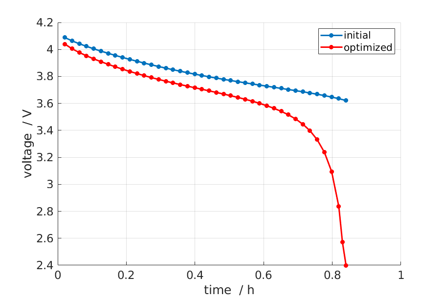
Finally we may plot the voltage curves to compare the result from the optimization procedure with the original.
 if doPlot
    % Plot
    figure; hold on; grid on
    E    = cellfun(@(x) x.Control.E, states);
    time = cellfun(@(x) x.time, states);
    plot(time/hour, E, '*-', 'displayname', 'initial');
    plot(time_opt/hour, E_opt, 'r*-', 'displayname', 'optimized');
    xlabel('time  / h');
    ylabel('voltage  / V');
    legend;
end
The result is shown in the figure below.