Thermal Simulation

BattMo support simulations with thermal coupling. Here, we look at the example given in runThermalExample

First we setup our model, in the same way as before, by merging different json inputs. We use a simple 3D model mainly used for demonstration.

%% Setup material properties

jsonfilename = fullfile('ParameterData'        , ...
                        'BatteryCellParameters', ...
                        'LithiumIonBatteryCell', ...
                        'lithium_ion_battery_nmc_graphite.json');
jsonstruct_material = parseBattmoJson(jsonfilename);

jsonstruct_material.include_current_collectors = true;

%% Setup geometry
jsonfilename = fullfile('Examples'     , ...
                        'JsonDataFiles', ...
                        'geometry3d.json');
jsonstruct_geometry = parseBattmoJson(jsonfilename);

%% Setup Control
jsonfilename = fullfile('Examples', 'JsonDataFiles', 'cc_discharge_control.json');
jsonstruct_control = parseBattmoJson(jsonfilename);

jsonstruct = mergeJsonStructs({jsonstruct_geometry , ...
                               jsonstruct_material , ...
                               jsonstruct_control});

%% Plot the extrnal heat transfer coefficient

model = setupModelFromJson(jsonstruct);

In the json structure lithium_ion_battery_nmc_graphite.json, the flag use_thermal is set to true, which means that the simulation will include thermal effects.

The thermal parameters are given for each component. They typically consists of

• Specific Heat Capacity

• Thermal Conducitivty

From those, we compute effective quantities. For the coating, it is done by processing the corresponding properties of the constituents. The effective thermal conductivity takes into account the volume fraction.

The parameters needed to compute the heat exchange with the exterior are

• The external temperature (K)

• The external heat transfer coefficient (W/m²/s)

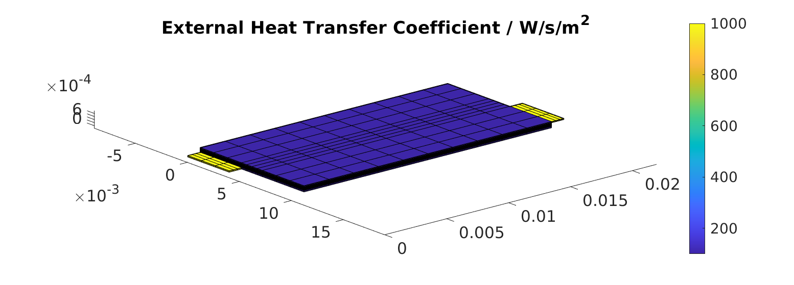
The external heat transfer coefficient can take different values for each external face of the model. It will then depend on the chosen geometrical domain. For our simple 3D model, the json interface gives us the possibility to set two values : A default value used for all external faces which is overwritten by the value given for the tabs. In our example we use 100 W/m²/s and 1000 W/m²/s, respectively.

Let us visualize those values. We run the following

% We index of the faces that are coupled to thermally to the exterior
extfaceind = model.ThermalModel.couplingTerm.couplingfaces;
G          = model.ThermalModel.grid;
nf         = G.faces.num;

% We create a vector with one value per face with value equal to the external heat transfer coefficient for the external
% face
val = NaN(nf, 1);
val(extfaceind) = model.ThermalModel.externalHeatTransferCoefficient;

figure
plotFaceData(G, val, 'edgecolor', 'black');
view([50, 50]);
title('External Heat Transfer Coefficient / W/s/m^2')
colorbar

and obtain

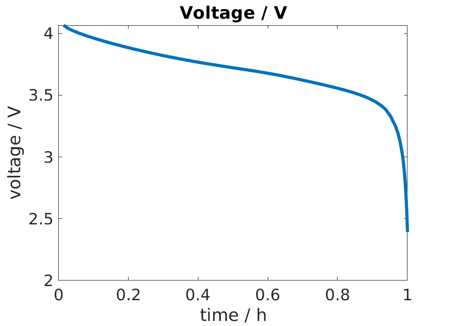
We run the simulation

output = runBatteryJson(jsonstruct);

We obtain the standard discharge curve

Then, we extract the temperature results and the minimum and maximum values from the output

Tabs = PhysicalConstants.Tabs;

states = output.states;

Tmin = cellfun(@(state) min(state.ThermalModel.T + Tabs), states);
Tmax = cellfun(@(state) max(state.ThermalModel.T + Tabs), states);

We plot those

figure
hold on
plot(time / hour, Tmin, 'displayname', 'min T');
plot(time / hour, Tmax, 'displayname', 'max T');
title('Temperature / C')
xlabel('time / h');
ylabel('Temperature / C');

legend show

and obtain

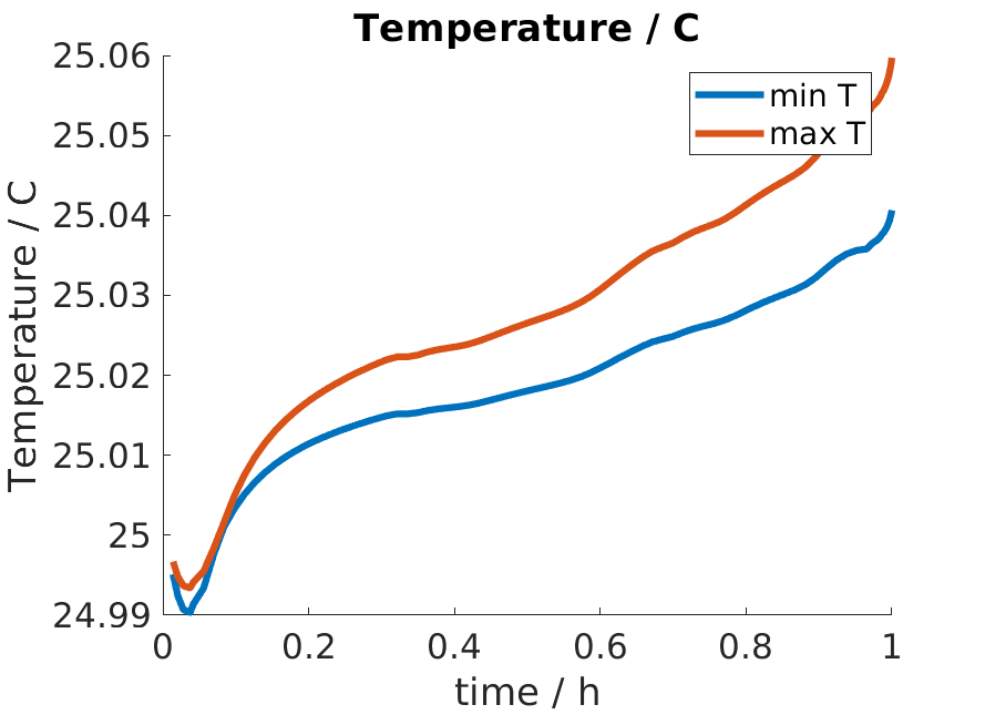
We notice that there is very little temperature variation. The reason is that we have a small cell which is very thin, with a lot of external contact where heat can be released.

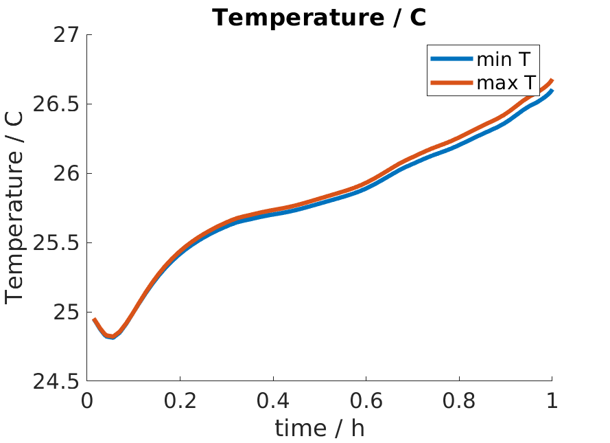
Let us use a different heat exchange coefficient. We set the default heat exchange to zero so that heat exchange can only occur through the tabs.

jsonstruct.ThermalModel.externalHeatTransferCoefficientTab = 100;
jsonstruct.ThermalModel.externalHeatTransferCoefficient = 0;

We run the computation again and obtain higher temperature.

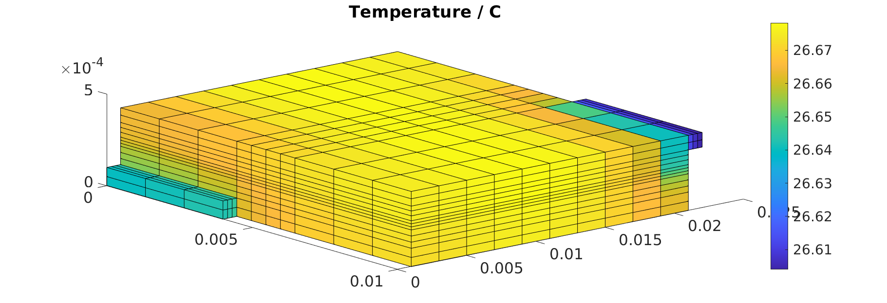
We have access to the temperature distribution for all the cells in the model. Let us plot the temperature field for the last time step. To do so, we run

state = states{end}
figure
plotCellData(model.ThermalModel.grid, ...
             state.ThermalModel.T + Tabs);
colorbar
title('Temperature / C');
view([50, 50]);

We obtain

The whole script can be viewed here.