Handling simulation outputs
In this tutorial we will explore the outputs of a simulation for interesting tasks:
Plot voltage and current curves
Plot overpotentials
Plot cell states in space and time
Save outputs
Load outputs.
Lets start with loading some pre-defined cell parameters, cycling protocols, and running a simulation.
using BattMo, GLMakie

cell_parameters = load_cell_parameters(; from_default_set = "Chen2020")
cycling_protocol = load_cycling_protocol(; from_default_set = "CCDischarge")

model_setup = LithiumIonBattery()

sim = Simulation(model_setup, cell_parameters, cycling_protocol);

output = solve(sim)
✔️ Validation of ModelSettings passed: No issues found.
──────────────────────────────────────────────────
✔️ Validation of CellParameters passed: No issues found.
──────────────────────────────────────────────────
✔️ Validation of CyclingProtocol passed: No issues found.
──────────────────────────────────────────────────
✔️ Validation of SimulationSettings passed: No issues found.
──────────────────────────────────────────────────
Jutul: Simulating 2 hours, 12 minutes as 163 report steps
╭────────────────┬───────────┬───────────────┬──────────╮
│ Iteration type │ Avg/step │ Avg/ministep │ Total │
│ │ 146 steps │ 146 ministeps │ (wasted) │
├────────────────┼───────────┼───────────────┼──────────┤
│ Newton │ 2.32877 │ 2.32877 │ 340 (0) │
│ Linearization │ 3.32877 │ 3.32877 │ 486 (0) │
│ Linear solver │ 2.32877 │ 2.32877 │ 340 (0) │
│ Precond apply │ 0.0 │ 0.0 │ 0 (0) │
╰────────────────┴───────────┴───────────────┴──────────╯
╭───────────────┬────────┬────────────┬──────────╮
│ Timing type │ Each │ Relative │ Total │
│ │ ms │ Percentage │ ms │
├───────────────┼────────┼────────────┼──────────┤
│ Properties │ 0.0349 │ 2.47 % │ 11.8830 │
│ Equations │ 0.5443 │ 55.03 % │ 264.5312 │
│ Assembly │ 0.0637 │ 6.44 % │ 30.9576 │
│ Linear solve │ 0.3318 │ 23.47 % │ 112.7972 │
│ Linear setup │ 0.0000 │ 0.00 % │ 0.0000 │
│ Precond apply │ 0.0000 │ 0.00 % │ 0.0000 │
│ Update │ 0.0455 │ 3.22 % │ 15.4711 │
│ Convergence │ 0.0640 │ 6.47 % │ 31.1073 │
│ Input/Output │ 0.0221 │ 0.67 % │ 3.2256 │
│ Other │ 0.0315 │ 2.23 % │ 10.7215 │
├───────────────┼────────┼────────────┼──────────┤
│ Total │ 1.4138 │ 100.00 % │ 480.6944 │
╰───────────────┴────────┴────────────┴──────────╯Now we'll have a look into what the output entail. The ouput is of type NamedTuple and contains multiple dicts. Lets print the keys of each dict.
keys(output)(:states, :cellSpecifications, :reports, :inputparams, :extra)So we can see the the output contains state data, cell specifications, reports on the simulation, the input parameters of the simulation, and some extra data. The most important dicts, that we'll dive a bit deeper into, are the states and cell specifications. First let's see how the states output is structured.
States
states = output[:states]
typeof(states)
Vector{OrderedDict{Symbol, Any}} (alias for Array{OrderedCollections.OrderedDict{Symbol, Any}, 1})As we can see, the states output is a Vector that contains dicts.
keys(states)145-element LinearIndices{1, Tuple{Base.OneTo{Int64}}}:
1
2
3
4
5
6
7
8
9
10
⋮
137
138
139
140
141
142
143
144
145In this case it consists of 77 dicts. Each dict represents a time step in the simulation and each time step stores quantities divided into battery component related group. This structure agrees with the overal model structure of BattMo.
initial_state = states[1]
keys(initial_state)
KeySet for a OrderedCollections.OrderedDict{Symbol, Any} with 5 entries. Keys:
:NeAm
:Elyte
:PeAm
:Control
:substatesSo each time step contains quantities related to the electrolyte, the negative electrode active material, the cycling control, and the positive electrode active material. Lets print the stored quantities for each group.
Electrolyte keys:
keys(initial_state[:Elyte])KeySet for a OrderedCollections.OrderedDict{Symbol, Any} with 6 entries. Keys:
:Phi
:C
:Charge
:Mass
:Conductivity
:DiffusivityNegative electrode active material keys:
keys(initial_state[:NeAm])KeySet for a OrderedCollections.OrderedDict{Symbol, Any} with 6 entries. Keys:
:Phi
:Cp
:Cs
:Charge
:Ocp
:TemperaturePositive electrode active material keys:
keys(initial_state[:PeAm])KeySet for a OrderedCollections.OrderedDict{Symbol, Any} with 6 entries. Keys:
:Phi
:Cp
:Cs
:Charge
:Ocp
:TemperatureControl keys:
keys(initial_state[:Control])KeySet for a OrderedCollections.OrderedDict{Symbol, Any} with 3 entries. Keys:
:Phi
:Current
:ControllerCell specifications
Now lets see what quantities are stored within the cellSpecifications dict in the simulation output.
cell_specifications = output[:cellSpecifications];
keys(cell_specifications)
KeySet for a Dict{Any, Any} with 4 entries. Keys:
"NegativeElectrodeCapacity"
"MaximumEnergy"
"PositiveElectrodeCapacity"
"Mass"Let's say we want to plot the cell current and cell voltage over time. First we'll retrieve these three quantities from the output.
states = output[:states]

t = [state[:Control][:Controller].time for state in states]
E = [state[:Control][:Phi][1] for state in states]
I = [state[:Control][:Current][1] for state in states]
Now we can use GLMakie to create a plot. Lets first plot the cell voltage.
f = Figure(size = (1000, 400))

ax = Axis(f[1, 1],
	title = "Voltage",
	xlabel = "Time / s",
	ylabel = "Voltage / V",
	xlabelsize = 25,
	ylabelsize = 25,
	xticklabelsize = 25,
	yticklabelsize = 25,
)


scatterlines!(ax,
	t,
	E;
	linewidth = 4,
	markersize = 10,
	marker = :cross,
	markercolor = :black,
)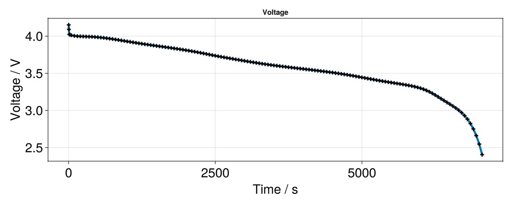
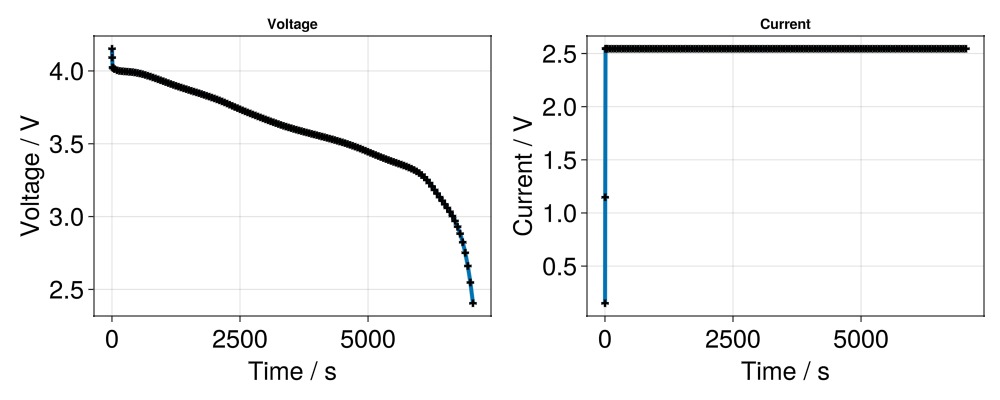
And the cell current.
ax = Axis(f[1, 2],
	title = "Current",
	xlabel = "Time / s",
	ylabel = "Current / V",
	xlabelsize = 25,
	ylabelsize = 25,
	xticklabelsize = 25,
	yticklabelsize = 25,
)


scatterlines!(ax,
	t,
	I;
	linewidth = 4,
	markersize = 10,
	marker = :cross,
	markercolor = :black,
)
Retrieving other quantities
Concentration
negative_electrode_surface_concentration = Array([[state[:NeAm][:Cs] for state in states]]);
positive_electrode_surface_concentration = Array([[state[:PeAm][:Cs] for state in states]]);
negative_electrode_particle_concentration = Array([[state[:NeAm][:Cp] for state in states]]);
positive_electrode_particle_concentration = Array([[state[:PeAm][:Cp] for state in states]]);
electrolyte_concentration = [state[:Elyte][:C] for state in states];
Potential
negative_electrode_potential = [state[:NeAm][:Phi] for state in states];
electrolyte_potential = [state[:Elyte][:Phi] for state in states];
positive_electrode_potential = [state[:PeAm][:Phi] for state in states];
Grid wrapper: We need Jutul to get the grid wrapper.
using Jutul

extra = output[:extra]
model = extra[:model]
negative_electrode_grid_wrap = physical_representation(model[:NeAm]);
electrolyte_grid_wrap = physical_representation(model[:Elyte]);
positive_electrode_grid_wrap = physical_representation(model[:PeAm]);
Mesh cell centroids coordinates
centroids_NeAm = negative_electrode_grid_wrap[:cell_centroids, Cells()];
centroids_Elyte = electrolyte_grid_wrap[:cell_centroids, Cells()];
print(centroids_Elyte)
centroids_PeAm = positive_electrode_grid_wrap[:cell_centroids, Cells()];
[4.259999999999998e-6 1.2780000000000001e-5 2.1299999999999993e-5 2.981999999999999e-5 3.834000000000001e-5 4.6859999999999975e-5 5.538e-5 6.39e-5 7.241999999999997e-5 8.094000000000001e-5 8.720000000000003e-5 9.119999999999998e-5 9.520000000000001e-5 0.00010098000000000003 0.00010854000000000003 0.00011610000000000004 0.00012366000000000002 0.00013122000000000003 0.00013878000000000002 0.00014634 0.00015389999999999995 0.00016146 0.00016901999999999998; 0.051350000000000014 0.05135000000000001 0.05134999999999999 0.05135000000000001 0.05135000000000001 0.05134999999999998 0.05135000000000002 0.051350000000000014 0.051350000000000014 0.051350000000000014 0.051350000000000014 0.05134999999999997 0.051350000000000014 0.051349999999999965 0.05134999999999999 0.05134999999999997 0.051349999999999965 0.05134999999999997 0.05134999999999998 0.05134999999999999 0.05134999999999998 0.05134999999999999 0.051349999999999986; 0.4999999999999998 0.4999999999999999 0.49999999999999983 0.5 0.5 0.49999999999999994 0.5000000000000002 0.5 0.5 0.5 0.5 0.49999999999999994 0.5 0.4999999999999998 0.5 0.4999999999999999 0.4999999999999998 0.4999999999999999 0.49999999999999994 0.4999999999999999 0.5 0.5 0.5000000000000001]Boundary faces coordinates
boundaries_NeAm = negative_electrode_grid_wrap[:boundary_centroids, BoundaryFaces()];
boundaries_Elyte = electrolyte_grid_wrap[:boundary_centroids, BoundaryFaces()];
boundaries_PeAm = positive_electrode_grid_wrap[:boundary_centroids, BoundaryFaces()];
UPDATE WITH NEW OUTPUT API
The simulation output
Access overpotentials
Plot cell states
Save and load outputs
Example on GitHub
If you would like to run this example yourself, it can be downloaded from the BattMo.jl GitHub repository as a script.
This page was generated using Literate.jl.