How to run a simulation

BattMo simulations replicates the voltage-current response of a cell. To run a Battmo simulation, the basic workflow is:

• Set up cell parameters

• Set up a cycling protocol

• Select a model

• Prepare a simulation

• Run the simulation

• Inspect and visualize the outputs of the simulation

To start, we load BattMo (battery models and simulations) and GLMakie (plotting).

using BattMo, GLMakie

BattMo stores cell parameters, cycling protocols and settings in a user-friendly JSON format to facilitate reuse. For our example, we read the cell parameter set from a NMC811 vs Graphite-SiOx cell whose parameters were determined in the Chen 2020 paper. We also read an example cycling protocol for a simple Constant Current Discharge.

cell_parameters = load_cell_parameters(; from_default_set = "Chen2020")
cycling_protocol = load_cycling_protocol(; from_default_set = "CCDischarge")

Next, we select the Lithium-Ion Battery Model with default model settings. A model can be thought as a mathematical implementation of the electrochemical and transport phenomena occuring in a real battery cell. The implementation consist of a system of partial differential equations and their corresponding parameters, constants and boundary conditions. The default Lithium-Ion Battery Model selected below corresponds to a basic P2D model, where neither current collectors nor thermal effects are considered.

model_setup = LithiumIonBattery()

LithiumIonBattery("Setup object for a P2D lithium-ion model", {
    "RampUp" => "Sinusoidal"
    "Metadata" =>     {
        "Description" => "Default model settings for a P2D simulation including a current ramp up, excluding current collectors and SEI effects."
        "Title" => "P2D"
    }
    "TransportInSolid" => "FullDiffusion"
    "ModelFramework" => "P2D"
}, true)

Then we setup a Simulation by passing the model, cell parameters and a cycling protocol. A Simulation can be thought as a procedure to predict how the cell responds to the cycling protocol, by solving the equations in the model using the cell parameters passed. We first prepare the simulation:

sim = Simulation(model_setup, cell_parameters, cycling_protocol);

✔️ Validation of CellParameters passed: No issues found.
──────────────────────────────────────────────────
✔️ Validation of CyclingProtocol passed: No issues found.
──────────────────────────────────────────────────
✔️ Validation of SimulationSettings passed: No issues found.
──────────────────────────────────────────────────

When the simulation is prepared, there are some validation checks happening in the background, which verify whether the cell parameters, cycling protocol and settings are sensible and complete to run a simulation. It is good practice to ensure that the Simulation has been properly configured by checking if has passed the validation procedure:

sim.is_valid

true

Now we can run the simulation

output = solve(sim;)

Jutul: Simulating 2 hours, 12 minutes as 163 report steps
╭────────────────┬───────────┬───────────────┬──────────╮
│ Iteration type │  Avg/step │  Avg/ministep │    Total │
│                │ 146 steps │ 146 ministeps │ (wasted) │
├────────────────┼───────────┼───────────────┼──────────┤
│ Newton         │   2.32877 │       2.32877 │  340 (0) │
│ Linearization  │   3.32877 │       3.32877 │  486 (0) │
│ Linear solver  │   2.32877 │       2.32877 │  340 (0) │
│ Precond apply  │       0.0 │           0.0 │    0 (0) │
╰────────────────┴───────────┴───────────────┴──────────╯
╭───────────────┬────────┬────────────┬──────────╮
│ Timing type   │   Each │   Relative │    Total │
│               │     ms │ Percentage │       ms │
├───────────────┼────────┼────────────┼──────────┤
│ Properties    │ 0.0382 │     1.34 % │  12.9882 │
│ Equations     │ 1.6404 │    82.37 % │ 797.2301 │
│ Assembly      │ 0.0712 │     3.58 % │  34.6204 │
│ Linear solve  │ 0.1683 │     5.91 % │  57.2203 │
│ Linear setup  │ 0.0000 │     0.00 % │   0.0000 │
│ Precond apply │ 0.0000 │     0.00 % │   0.0000 │
│ Update        │ 0.0506 │     1.78 % │  17.1883 │
│ Convergence   │ 0.0688 │     3.46 % │  33.4483 │
│ Input/Output  │ 0.0244 │     0.37 % │   3.5682 │
│ Other         │ 0.0340 │     1.19 % │  11.5622 │
├───────────────┼────────┼────────────┼──────────┤
│ Total         │ 2.8465 │   100.00 % │ 967.8260 │
╰───────────────┴────────┴────────────┴──────────╯

The ouput is a NamedTuple storing the results of the simulation within multiple dictionaries. Let's plot the cell current and cell voltage over time and make a plot with the GLMakie package.

states = output[:states]

t = [state[:Control][:Controller].time for state in states]
E = [state[:Control][:Phi][1] for state in states]
I = [state[:Control][:Current][1] for state in states]


f = Figure(size = (1000, 400))

ax = Axis(f[1, 1], title = "Voltage", xlabel = "Time / s", ylabel = "Voltage / V",
	xlabelsize = 25,
	ylabelsize = 25,
	xticklabelsize = 25,
	yticklabelsize = 25,
)
scatterlines!(ax, t, E; linewidth = 4, markersize = 10, marker = :cross, markercolor = :black)

f

ax = Axis(f[1, 2], title = "Current", xlabel = "Time / s", ylabel = "Current / V",
	xlabelsize = 25,
	ylabelsize = 25,
	xticklabelsize = 25,
	yticklabelsize = 25,
)
scatterlines!(ax, t, I; linewidth = 4, markersize = 10, marker = :cross, markercolor = :black)

f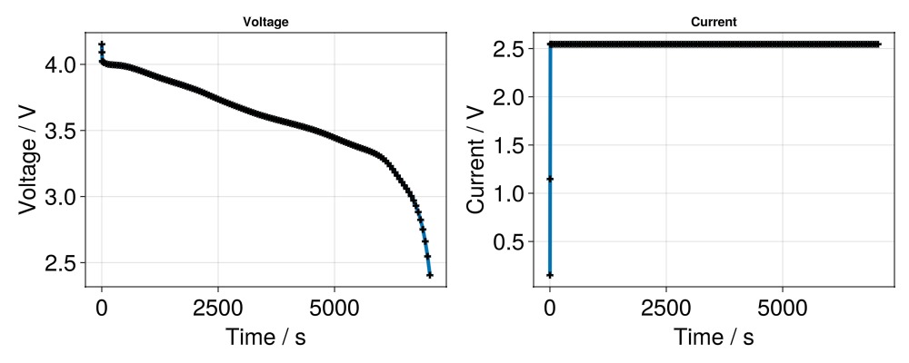

Example on GitHub

If you would like to run this example yourself, it can be downloaded from the BattMo.jl GitHub repository as a script.

---

This page was generated using Literate.jl.