Example of jelly roll

This example demonstrates how to set up, run and visualize a 3D cylindrical battery model

Load the packages

using BattMo, GLMakie, Jutul

Load the cell parameters

cell_parameters     = load_cell_parameters(; from_default_set = "Chen2020")
cycling_protocol    = load_cycling_protocol(; from_default_set = "CCDischarge")
model_settings      = load_model_settings(; from_default_set = "P4D_cylindrical")
simulation_settings = load_simulation_settings(; from_default_set = "P4D_cylindrical")

Set up the model

model_setup = LithiumIonBattery(; model_settings)

✔️ Validation of ModelSettings passed: No issues found.
──────────────────────────────────────────────────

Review and modify the cell parameters

We go through some of the geometrical and discretization parameters. We modify some of them to obtain a cell where the different components are easier to visualize

The cell geometry is determined by the inner and outer radius and the height. We reduce the outer radius

cell_parameters["Cell"]["OuterRadius"] = 0.010

We modify the current collector thicknesses, for visualization purpose

cell_parameters["NegativeElectrode"]["CurrentCollector"]["Thickness"]    = 50e-6
cell_parameters["PositiveElectrode"]["CurrentCollector"]["Thickness"]    = 50e-6

The tabs are part of the current collectors that connect the electrodes to the external circuit. The location of the tabs is given as a fraction length, where the length is measured along the current collector in the horizontal direction, meaning that we follow the rolling spiral. Indeed, this is the relevant length to use if we want to dispatch the current collector in a equilibrated way, where each of them will a priori collect the same amount of current. In the following, we include three tabs with one in the middle and the other at a distance such that each tab will collect one third of the current

cell_parameters["NegativeElectrode"]["CurrentCollector"]["TabFractions"] = [0.5/3, 0.5, 0.5 + 0.5/3]
cell_parameters["PositiveElectrode"]["CurrentCollector"]["TabFractions"] = [0.5/3, 0.5, 0.5 + 0.5/3]

We set the tab width to 2 mm

cell_parameters["NegativeElectrode"]["CurrentCollector"]["TabWidth"] = 0.002
cell_parameters["PositiveElectrode"]["CurrentCollector"]["TabWidth"] = 0.002

The angular discretization of the cell is determined by the number of angular grid points.

simulation_settings["GridResolution"]["Angular"] = 30

Create the simulation object

sim = Simulation(model_setup, cell_parameters, cycling_protocol; simulation_settings);

✔️ Validation of CellParameters passed: No issues found.
──────────────────────────────────────────────────
✔️ Validation of CyclingProtocol passed: No issues found.
──────────────────────────────────────────────────
✔️ Validation of SimulationSettings passed: No issues found.
──────────────────────────────────────────────────

We preprocess the simulation object to retrieve the grids and coupling structure, which we want to visualize prior running the simulation

output = get_simulation_input(sim)
grids     = output[:grids]
couplings = output[:couplings]

Visualize the grids and couplings

Define a list of the component to iterate over in the ploting routin below

components = ["NegativeElectrode", "PositiveElectrode", "NegativeCurrentCollector", "PositiveCurrentCollector" ]
colors = [:gray, :green, :blue, :black]

We plot the components

for (i, component) in enumerate(components)
    if i == 1
        global fig, ax = plot_mesh(grids[component],
                            color = colors[i])
    else
        plot_mesh!(ax,
                   grids[component],
                   color = colors[i])
    end
end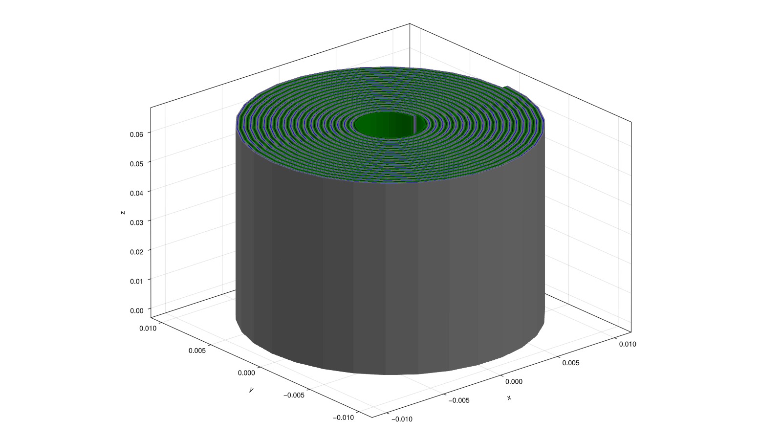

Plot the current collectors tabs

We plot the tabs, which couple the current collectors with the external circuits. The tabs will typically protude from the cell in the vertical directions but we can neglect this 3d feature in the simulation model. The tabs are then represented by horizontal faces at the top or bottom of the current collectors. In the figure below, they are plotted in red.

components = [
    "NegativeCurrentCollector",
    "PositiveCurrentCollector"
]

for component in components
    plot_mesh!(ax, grids[component];
               boundaryfaces = couplings[component]["External"]["boundaryfaces"],
               color = :red)
end


ax.azimuth[] = 4.0
ax.elevation[] = 1.56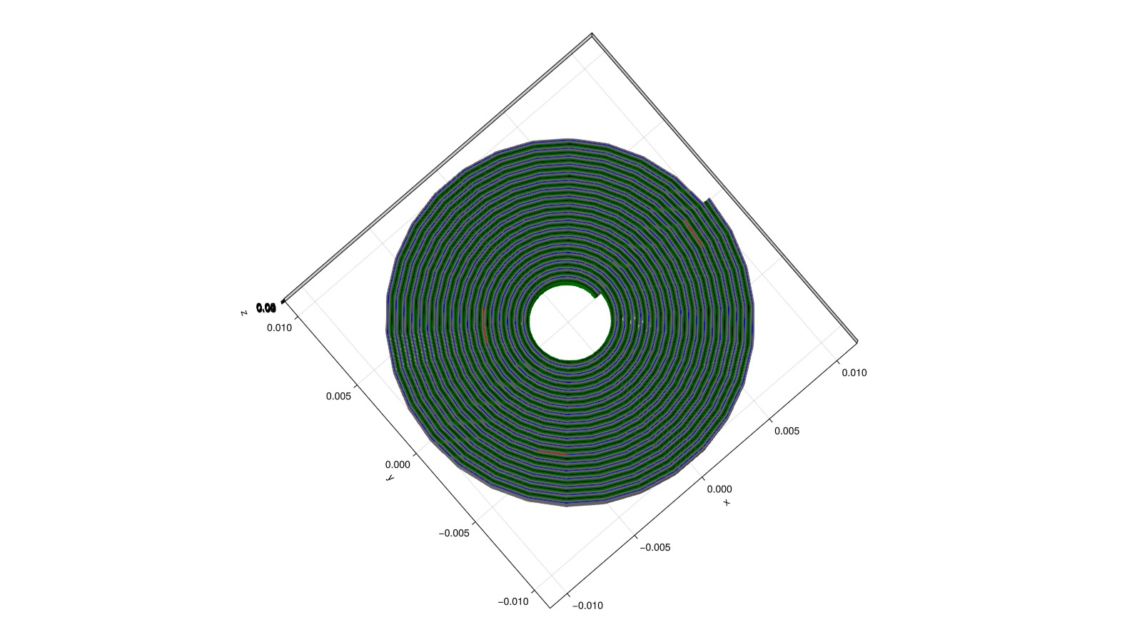

Simulation

We reload the original parameters

cell_parameters     = load_cell_parameters(; from_default_set = "Chen2020")
cycling_protocol    = load_cycling_protocol(; from_default_set = "CCDischarge")
model_settings      = load_model_settings(; from_default_set = "P4D_cylindrical")
simulation_settings = load_simulation_settings(; from_default_set = "P4D_cylindrical")

{
    "GridResolution" =>     {
        "PositiveElectrodeCoating" => 3
        "Separator" => 3
        "NegativeElectrodeActiveMaterial" => 5
        "NegativeElectrodeCoating" => 3
        "NegativeElectrodeCurrentCollector" => 3
        "Angular" => 8
        "Height" => 2
        "PositiveElectrodeCurrentCollector" => 3
        "PositiveElectrodeCurrentCollectorTabWidth" => 2
        "PositiveElectrodeActiveMaterial" => 5
        "NegativeElectrodeCurrentCollectorTabWidth" => 2
    }
    "TimeStepDuration" => 50
    "RampUpTime" => 10
    "RampUpSteps" => 5
}

We adjust the parameters so that the simulation in this example is not too long (around a couple of minutes)

cell_parameters["Cell"]["OuterRadius"] = 0.004
cell_parameters["NegativeElectrode"]["CurrentCollector"]["TabFractions"] = [0.5]
cell_parameters["PositiveElectrode"]["CurrentCollector"]["TabFractions"] = [0.5]
cell_parameters["NegativeElectrode"]["CurrentCollector"]["TabWidth"]     = 0.002
cell_parameters["PositiveElectrode"]["CurrentCollector"]["TabWidth"]     = 0.002
simulation_settings["GridResolution"]["Angular"] = 8

8

We setup the simulation and run it

sim = Simulation(model_setup, cell_parameters, cycling_protocol; simulation_settings);
output = solve(sim; info_level = -1)

✔️ Validation of CellParameters passed: No issues found.
──────────────────────────────────────────────────
✔️ Validation of CyclingProtocol passed: No issues found.
──────────────────────────────────────────────────
✔️ Validation of SimulationSettings passed: No issues found.
──────────────────────────────────────────────────

Visualization of the simulation output

We plot the discharge curve

states = output[:states]
model  = output[:extra][:model]

t = [state[:Control][:Controller].time for state in states]
E = [state[:Control][:Phi][1] for state in states]
I = [state[:Control][:Current][1] for state in states]

f = Figure(size = (1000, 400))

ax = Axis(f[1, 1],
	title = "Voltage",
	xlabel = "Time / s",
	ylabel = "Voltage / V",
	xlabelsize = 25,
	ylabelsize = 25,
	xticklabelsize = 25,
	yticklabelsize = 25)

scatterlines!(ax,
	t,
	E;
	linewidth = 4,
	markersize = 10,
	marker = :cross,
	markercolor = :black,
)

ax = Axis(f[1, 2],
	title = "Current",
	xlabel = "Time / s",
	ylabel = "Current / A",
	xlabelsize = 25,
	ylabelsize = 25,
	xticklabelsize = 25,
	yticklabelsize = 25,
)

scatterlines!(ax,
	t,
	I;
	linewidth = 4,
	markersize = 10,
	marker = :cross,
	markercolor = :black)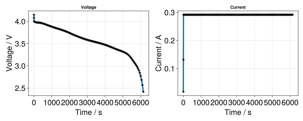

We open the interactive visualization tool with the simulation output.

plot_interactive_3d(output; colormap = :curl)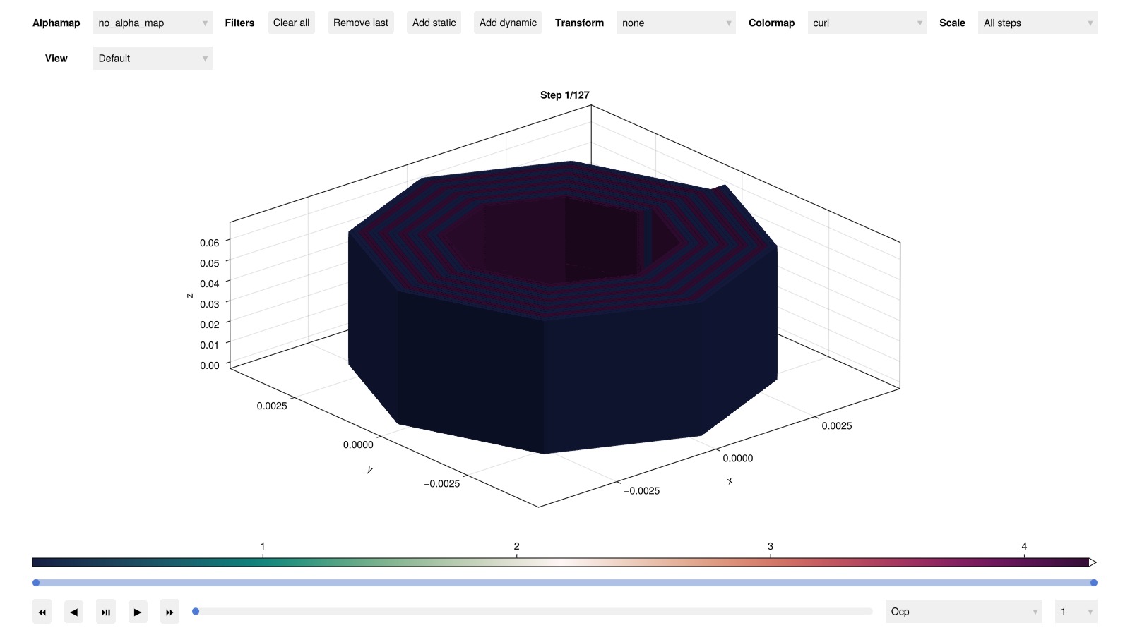

Example on GitHub

If you would like to run this example yourself, it can be downloaded from the BattMo.jl GitHub repository as a script.

---

This page was generated using Literate.jl.