Gradient-based parameter calibration of a lithium-ion battery model
This example demonstrates how to calibrate a lithium-ion battery against data model using BattMo.jl. The example uses a two-step calibration process:
We first calibrate the model against a 0.5C discharge curve (adjusting stoichiometric coefficients and maximum concentration in the active material)
We then calibrate the model against a 2.0C discharge curve (adjusting reaction rate constants and diffusion coefficients in the active material)
Finally, we compare the results of the calibrated model against the experimental data for discharge rates of 0.5C, 1.0C, and 2.0C.
Load packages and set up helper functions
using BattMo, Jutul
using CSV
using DataFrames
using GLMakie

function get_tV(x)
    t = [state[:Control][:Controller].time for state in x[:states]]
    V = [state[:Control][:Phi][1] for state in x[:states]]
    return (t, V)
end

function get_tV(x::DataFrame)
    return (x[:, 1], x[:, 2])
end
get_tV (generic function with 2 methods)Load the experimental data and set up a base case
battmo_base = normpath(joinpath(pathof(BattMo) |> splitdir |> first, ".."))
exdata = joinpath(battmo_base, "examples", "example_data")
df_05 = CSV.read(joinpath(exdata, "Xu_2015_voltageCurve_05C.csv"), DataFrame)
df_1 = CSV.read(joinpath(exdata, "Xu_2015_voltageCurve_1C.csv"), DataFrame)
df_2 = CSV.read(joinpath(exdata, "Xu_2015_voltageCurve_2C.csv"), DataFrame)

dfs = [df_05, df_1, df_2]

cell_parameters = load_cell_parameters(; from_default_set = "Xu2015")
cycling_protocol = load_cycling_protocol(; from_default_set = "CCDischarge")

cycling_protocol["LowerVoltageLimit"] = 2.25
model_setup = LithiumIonBattery()

cycling_protocol["DRate"] = 0.5
sim = Simulation(model_setup, cell_parameters, cycling_protocol)
output0 = solve(sim)

t0, V0 = get_tV(output0)
t_exp_05, V_exp_05 = get_tV(df_05)
t_exp_1, V_exp_1 = get_tV(df_1)

fig = Figure()
ax = Axis(fig[1, 1], title = "CRate = 0.5", xlabel = "Time / s", ylabel = "Voltage / V")
lines!(ax, t0, V0, label = "Base case")
lines!(ax, t_exp_05, V_exp_05, label = "Experimental data")
axislegend(position = :lb)
fig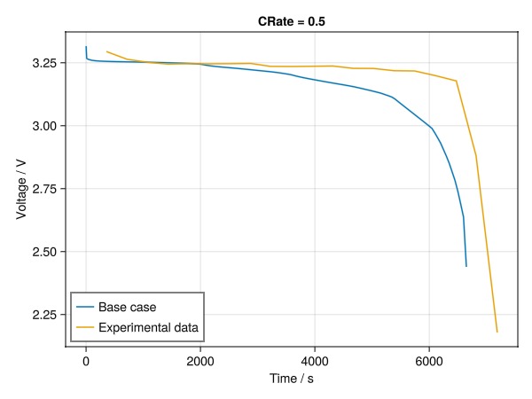
Set up the first calibration
We select the following parameters to calibrate:
"StoichiometricCoefficientAtSOC100" at both electrodes
"StoichiometricCoefficientAtSOC0" at both electrodes
"MaximumConcentration" of both electrodes
We also set bounds for these parameters to ensure they remain physically meaningful and possible to simulate. The objective function is the sum of squares:
We print the setup as a table to give the user the opportunity to review the setup before calibration starts.
vc05 = VoltageCalibration(t_exp_05, V_exp_05, sim)

free_calibration_parameter!(vc05,
    ["NegativeElectrode","ActiveMaterial", "StoichiometricCoefficientAtSOC100"];
    lower_bound = 0.0, upper_bound = 1.0)
free_calibration_parameter!(vc05,
    ["PositiveElectrode","ActiveMaterial", "StoichiometricCoefficientAtSOC100"];
    lower_bound = 0.0, upper_bound = 1.0)
VoltageCalibration([357.76627218934914, 715.9763313609469, 1074.1863905325445, 1432.396449704142, 1790.6065088757396, 2148.816568047337, 2507.0266272189347, 2877.5887573964496, 3223.44674556213, 3594.0088757396447, 3952.2189349112427, 4310.42899408284, 4668.639053254437, 5026.8491124260345, 5385.059171597633, 5743.2692307692305, 6101.479289940828, 6472.041420118343, 6817.899408284024, 7188.461538461537], [3.2943262673632967, 3.2638600156322126, 3.2518999695748874, 3.2446281622882482, 3.246486083133996, 3.245753135185418, 3.246253934281757, 3.2472569925301102, 3.2356583102522136, 3.2351808720466657, 3.2359284205519883, 3.237169467875278, 3.227800290612279, 3.2273140920726844, 3.2184384136276525, 3.217458716270091, 3.1992065602836877, 3.177878797019038, 2.8807910485472883, 2.179051790010771], Simulation(BattMo.run_battery, LithiumIonBattery("Setup object for a P2D lithium-ion model", {
"RampUp" => "Sinusoidal"
"Metadata" => {
"Description" => "Default model settings for a P2D simulation including a current ramp up, excluding current collectors and SEI effects."
"Title" => "P2D"
}
"TransportInSolid" => "FullDiffusion"
"ModelFramework" => "P2D"
}, true), {
"Electrolyte" => {
"TransferenceNumber" => 0.2594
"Description" => "1.5 mol/l LiPF6 dissolved in a mixture of ethylene carbonate (EC): dimethyl carbonate (DMC) (1:1)"
"DiffusionCoefficient" => "8.794*10^(-11)*(c/1000)^2 - 3.972*10^(-10)*(c/1000) + 4.862*10^(-10)"
"IonicConductivity" => "0.1297*(c/1000)^3 - 2.51*(c/1000)^(1.5) + 3.329*(c/1000)"
"Density" => 1210
"ChargeNumber" => 1
"Concentration" => 1500.0
}
"Cell" => {
"ElectrodeGeometricSurfaceArea" => 0.007035
"NominalCapacity" => 16.5
"ElectrodeWidth" => 0.067
"ElectrodeLength" => 0.105
"Name" => "LP2770120"
"Case" => "Pouch"
"NominalVoltage" => 3.2
}
"Metadata" => {
"Description" => "Parameter set of a commercial Type LP2770120 prismatic LiFePO4/graphite cell, for an electrochemical pseudo-two-dimensional (P2D) model."
"Source" => "https://doi.org/10.1016/j.energy.2014.11.073"
"Models" => {
"CurrentCollectors" => "Generic"
"RampUp" => "Sinusoidal"
"TransportInSolid" => "FullDiffusion"
"ModelFramework" => Any["P2D", "P4D Pouch"]
}
"Title" => "Xu2015"
}
"PositiveElectrode" => {
"ActiveMaterial" => {
"ActivationEnergyOfDiffusion" => 20000
"NumberOfElectronsTransfered" => 1
"StoichiometricCoefficientAtSOC0" => 0.999
"OpenCircuitPotential" => {
"FilePath" => "function_parameters_Xu2015.jl"
"FunctionName" => "open_circuit_potential_lfp_Xu_2015"
}
"ReactionRateConstant" => 3.626e-11
"MassFraction" => 1.0
"StoichiometricCoefficientAtSOC100" => 0.14778
"ActivationEnergyOfReaction" => 4000
"MaximumConcentration" => 26390
"VolumetricSurfaceArea" => 1.87826e6
"Description" => "LiFePO4"
"DiffusionCoefficient" => 1.25e-15
"ParticleRadius" => 1.15e-6
"Density" => 1500
"ElectronicConductivity" => 0.01
"ChargeTransferCoefficient" => 0.5
}
"ElectrodeCoating" => {
"BruggemanCoefficient" => 1.5
"EffectiveDensity" => 1080
"Thickness" => 9.2e-5
}
"Binder" => {
"Description" => "Unknown"
"MassFraction" => 0.0
"Density" => 1100.0
"ElectronicConductivity" => 100.0
}
"CurrentCollector" => {
"Description" => "Aluminum"
"TabLength" => 0.01
"Density" => 2700
"ElectronicConductivity" => 3.83e7
"Thickness" => 1.6e-5
"TabWidth" => 0.015
}
"ConductiveAdditive" => {
"Description" => "Unknown"
"MassFraction" => 0.0
"Density" => 1950.0
"ElectronicConductivity" => 100.0
}
}
"Separator" => {
"Density" => 779
"BruggemanCoefficient" => 1.5
"Thickness" => 2.0e-5
"Porosity" => 0.4
}
"NegativeElectrode" => {
"ActiveMaterial" => {
"ActivationEnergyOfDiffusion" => 4000
"NumberOfElectronsTransfered" => 1
"StoichiometricCoefficientAtSOC0" => 0.001
"OpenCircuitPotential" => {
"FilePath" => "function_parameters_Xu2015.jl"
"FunctionName" => "open_circuit_potential_graphite_Xu_2015"
}
"ReactionRateConstant" => 1.764e-11
"MassFraction" => 1.0
"StoichiometricCoefficientAtSOC100" => 0.51873811
"ActivationEnergyOfReaction" => 4000
"MaximumConcentration" => 31540
"VolumetricSurfaceArea" => 142373
"Description" => "Graphite"
"DiffusionCoefficient" => 3.9e-14
"ParticleRadius" => 1.475e-5
"Density" => 2660
"ElectronicConductivity" => 215.0
"ChargeTransferCoefficient" => 0.5
}
"ElectrodeCoating" => {
"BruggemanCoefficient" => 1.5
"EffectiveDensity" => 1862
"Thickness" => 5.9e-5
}
"Binder" => {
"Description" => "Unknown"
"MassFraction" => 0.0
"Density" => 1100.0
"ElectronicConductivity" => 100.0
}
"CurrentCollector" => {
"Description" => "Copper"
"TabLength" => 0.01
"Density" => 8900
"ElectronicConductivity" => 6.33e7
"Thickness" => 9.0e-6
"TabWidth" => 0.015
}
"ConductiveAdditive" => {
"Description" => "Unknown"
"MassFraction" => 0.0
"Density" => 1950.0
"ElectronicConductivity" => 100.0
}
}
}, {
"TotalNumberOfCycles" => 0
"InitialControl" => "discharging"
"InitialStateOfCharge" => 0.99
"InitialTemperature" => 298.15
"Metadata" => {
"Description" => "Parameter set for a constant current discharging protocol."
"Title" => "CCDischarge"
}
"DRate" => 0.5
"LowerVoltageLimit" => 2.25
"Protocol" => "CC"
"UpperVoltageLimit" => 4.1
}, {
"Grid" => Any[]
"GridResolution" => {
"PositiveElectrodeCoating" => 10
"Separator" => 3
"NegativeElectrodeActiveMaterial" => 5
"PositiveElectrodeCurrentCollectorTabLength" => 3
"NegativeElectrodeCoating" => 10
"NegativeElectrodeCurrentCollector" => 2
"ElectrodeLength" => 10
"NegativeElectrodeCurrentCollectorTabLength" => 3
"PositiveElectrodeCurrentCollector" => 2
"PositiveElectrodeCurrentCollectorTabWidth" => 3
"ElectrodeWidth" => 10
"PositiveElectrodeActiveMaterial" => 5
"NegativeElectrodeCurrentCollectorTabWidth" => 3
}
"TimeStepDuration" => 50
"RampUpTime" => 10
"RampUpSteps" => 5
}, true), {
["NegativeElectrode", "ActiveMaterial", "StoichiometricCoefficientAtSOC100"] => (v0 = 0.51873811, vmin = 0.0, vmax = 1.0)
["PositiveElectrode", "ActiveMaterial", "StoichiometricCoefficientAtSOC100"] => (v0 = 0.14778, vmin = 0.0, vmax = 1.0)
}, missing, missing)"StoichiometricCoefficientAtSOC0" at both electrodes
free_calibration_parameter!(vc05,
    ["NegativeElectrode","ActiveMaterial", "StoichiometricCoefficientAtSOC0"];
    lower_bound = 0.0, upper_bound = 1.0)
free_calibration_parameter!(vc05,
    ["PositiveElectrode","ActiveMaterial", "StoichiometricCoefficientAtSOC0"];
    lower_bound = 0.0, upper_bound = 1.0)
VoltageCalibration([357.76627218934914, 715.9763313609469, 1074.1863905325445, 1432.396449704142, 1790.6065088757396, 2148.816568047337, 2507.0266272189347, 2877.5887573964496, 3223.44674556213, 3594.0088757396447, 3952.2189349112427, 4310.42899408284, 4668.639053254437, 5026.8491124260345, 5385.059171597633, 5743.2692307692305, 6101.479289940828, 6472.041420118343, 6817.899408284024, 7188.461538461537], [3.2943262673632967, 3.2638600156322126, 3.2518999695748874, 3.2446281622882482, 3.246486083133996, 3.245753135185418, 3.246253934281757, 3.2472569925301102, 3.2356583102522136, 3.2351808720466657, 3.2359284205519883, 3.237169467875278, 3.227800290612279, 3.2273140920726844, 3.2184384136276525, 3.217458716270091, 3.1992065602836877, 3.177878797019038, 2.8807910485472883, 2.179051790010771], Simulation(BattMo.run_battery, LithiumIonBattery("Setup object for a P2D lithium-ion model", {
"RampUp" => "Sinusoidal"
"Metadata" => {
"Description" => "Default model settings for a P2D simulation including a current ramp up, excluding current collectors and SEI effects."
"Title" => "P2D"
}
"TransportInSolid" => "FullDiffusion"
"ModelFramework" => "P2D"
}, true), {
"Electrolyte" => {
"TransferenceNumber" => 0.2594
"Description" => "1.5 mol/l LiPF6 dissolved in a mixture of ethylene carbonate (EC): dimethyl carbonate (DMC) (1:1)"
"DiffusionCoefficient" => "8.794*10^(-11)*(c/1000)^2 - 3.972*10^(-10)*(c/1000) + 4.862*10^(-10)"
"IonicConductivity" => "0.1297*(c/1000)^3 - 2.51*(c/1000)^(1.5) + 3.329*(c/1000)"
"Density" => 1210
"ChargeNumber" => 1
"Concentration" => 1500.0
}
"Cell" => {
"ElectrodeGeometricSurfaceArea" => 0.007035
"NominalCapacity" => 16.5
"ElectrodeWidth" => 0.067
"ElectrodeLength" => 0.105
"Name" => "LP2770120"
"Case" => "Pouch"
"NominalVoltage" => 3.2
}
"Metadata" => {
"Description" => "Parameter set of a commercial Type LP2770120 prismatic LiFePO4/graphite cell, for an electrochemical pseudo-two-dimensional (P2D) model."
"Source" => "https://doi.org/10.1016/j.energy.2014.11.073"
"Models" => {
"CurrentCollectors" => "Generic"
"RampUp" => "Sinusoidal"
"TransportInSolid" => "FullDiffusion"
"ModelFramework" => Any["P2D", "P4D Pouch"]
}
"Title" => "Xu2015"
}
"PositiveElectrode" => {
"ActiveMaterial" => {
"ActivationEnergyOfDiffusion" => 20000
"NumberOfElectronsTransfered" => 1
"StoichiometricCoefficientAtSOC0" => 0.999
"OpenCircuitPotential" => {
"FilePath" => "function_parameters_Xu2015.jl"
"FunctionName" => "open_circuit_potential_lfp_Xu_2015"
}
"ReactionRateConstant" => 3.626e-11
"MassFraction" => 1.0
"StoichiometricCoefficientAtSOC100" => 0.14778
"ActivationEnergyOfReaction" => 4000
"MaximumConcentration" => 26390
"VolumetricSurfaceArea" => 1.87826e6
"Description" => "LiFePO4"
"DiffusionCoefficient" => 1.25e-15
"ParticleRadius" => 1.15e-6
"Density" => 1500
"ElectronicConductivity" => 0.01
"ChargeTransferCoefficient" => 0.5
}
"ElectrodeCoating" => {
"BruggemanCoefficient" => 1.5
"EffectiveDensity" => 1080
"Thickness" => 9.2e-5
}
"Binder" => {
"Description" => "Unknown"
"MassFraction" => 0.0
"Density" => 1100.0
"ElectronicConductivity" => 100.0
}
"CurrentCollector" => {
"Description" => "Aluminum"
"TabLength" => 0.01
"Density" => 2700
"ElectronicConductivity" => 3.83e7
"Thickness" => 1.6e-5
"TabWidth" => 0.015
}
"ConductiveAdditive" => {
"Description" => "Unknown"
"MassFraction" => 0.0
"Density" => 1950.0
"ElectronicConductivity" => 100.0
}
}
"Separator" => {
"Density" => 779
"BruggemanCoefficient" => 1.5
"Thickness" => 2.0e-5
"Porosity" => 0.4
}
"NegativeElectrode" => {
"ActiveMaterial" => {
"ActivationEnergyOfDiffusion" => 4000
"NumberOfElectronsTransfered" => 1
"StoichiometricCoefficientAtSOC0" => 0.001
"OpenCircuitPotential" => {
"FilePath" => "function_parameters_Xu2015.jl"
"FunctionName" => "open_circuit_potential_graphite_Xu_2015"
}
"ReactionRateConstant" => 1.764e-11
"MassFraction" => 1.0
"StoichiometricCoefficientAtSOC100" => 0.51873811
"ActivationEnergyOfReaction" => 4000
"MaximumConcentration" => 31540
"VolumetricSurfaceArea" => 142373
"Description" => "Graphite"
"DiffusionCoefficient" => 3.9e-14
"ParticleRadius" => 1.475e-5
"Density" => 2660
"ElectronicConductivity" => 215.0
"ChargeTransferCoefficient" => 0.5
}
"ElectrodeCoating" => {
"BruggemanCoefficient" => 1.5
"EffectiveDensity" => 1862
"Thickness" => 5.9e-5
}
"Binder" => {
"Description" => "Unknown"
"MassFraction" => 0.0
"Density" => 1100.0
"ElectronicConductivity" => 100.0
}
"CurrentCollector" => {
"Description" => "Copper"
"TabLength" => 0.01
"Density" => 8900
"ElectronicConductivity" => 6.33e7
"Thickness" => 9.0e-6
"TabWidth" => 0.015
}
"ConductiveAdditive" => {
"Description" => "Unknown"
"MassFraction" => 0.0
"Density" => 1950.0
"ElectronicConductivity" => 100.0
}
}
}, {
"TotalNumberOfCycles" => 0
"InitialControl" => "discharging"
"InitialStateOfCharge" => 0.99
"InitialTemperature" => 298.15
"Metadata" => {
"Description" => "Parameter set for a constant current discharging protocol."
"Title" => "CCDischarge"
}
"DRate" => 0.5
"LowerVoltageLimit" => 2.25
"Protocol" => "CC"
"UpperVoltageLimit" => 4.1
}, {
"Grid" => Any[]
"GridResolution" => {
"PositiveElectrodeCoating" => 10
"Separator" => 3
"NegativeElectrodeActiveMaterial" => 5
"PositiveElectrodeCurrentCollectorTabLength" => 3
"NegativeElectrodeCoating" => 10
"NegativeElectrodeCurrentCollector" => 2
"ElectrodeLength" => 10
"NegativeElectrodeCurrentCollectorTabLength" => 3
"PositiveElectrodeCurrentCollector" => 2
"PositiveElectrodeCurrentCollectorTabWidth" => 3
"ElectrodeWidth" => 10
"PositiveElectrodeActiveMaterial" => 5
"NegativeElectrodeCurrentCollectorTabWidth" => 3
}
"TimeStepDuration" => 50
"RampUpTime" => 10
"RampUpSteps" => 5
}, true), {
["PositiveElectrode", "ActiveMaterial", "StoichiometricCoefficientAtSOC0"] => (v0 = 0.999, vmin = 0.0, vmax = 1.0)
["NegativeElectrode", "ActiveMaterial", "StoichiometricCoefficientAtSOC100"] => (v0 = 0.51873811, vmin = 0.0, vmax = 1.0)
["PositiveElectrode", "ActiveMaterial", "StoichiometricCoefficientAtSOC100"] => (v0 = 0.14778, vmin = 0.0, vmax = 1.0)
["NegativeElectrode", "ActiveMaterial", "StoichiometricCoefficientAtSOC0"] => (v0 = 0.001, vmin = 0.0, vmax = 1.0)
}, missing, missing)"MaximumConcentration" of both electrodes
free_calibration_parameter!(vc05,
    ["NegativeElectrode","ActiveMaterial", "MaximumConcentration"];
    lower_bound = 10000.0, upper_bound = 1e5)
free_calibration_parameter!(vc05,
    ["PositiveElectrode","ActiveMaterial", "MaximumConcentration"];
    lower_bound = 10000.0, upper_bound = 1e5)

print_calibration_overview(vc05)
NegativeElectrode: Active calibration parameters
┌──────────────────────────────────────────────────┬───────────────┬────────────────────┐
│ Name │ Initial value │ Bounds │
├──────────────────────────────────────────────────┼───────────────┼────────────────────┤
│ ActiveMaterial.MaximumConcentration │ 31540 │ 10000.0 - 100000.0 │
│ ActiveMaterial.StoichiometricCoefficientAtSOC100 │ 0.518738 │ 0.0 - 1.0 │
│ ActiveMaterial.StoichiometricCoefficientAtSOC0 │ 0.001 │ 0.0 - 1.0 │
└──────────────────────────────────────────────────┴───────────────┴────────────────────┘
PositiveElectrode: Active calibration parameters
┌──────────────────────────────────────────────────┬───────────────┬────────────────────┐
│ Name │ Initial value │ Bounds │
├──────────────────────────────────────────────────┼───────────────┼────────────────────┤
│ ActiveMaterial.MaximumConcentration │ 26390 │ 10000.0 - 100000.0 │
│ ActiveMaterial.StoichiometricCoefficientAtSOC0 │ 0.999 │ 0.0 - 1.0 │
│ ActiveMaterial.StoichiometricCoefficientAtSOC100 │ 0.14778 │ 0.0 - 1.0 │
└──────────────────────────────────────────────────┴───────────────┴────────────────────┘Solve the first calibration problem
The calibration is performed by solving the optimization problem. This makes use of the adjoint method implemented in Jutul.jl and the LBFGS algorithm.
solve(vc05);
cell_parameters_calibrated = vc05.calibrated_cell_parameters;
print_calibration_overview(vc05)
Calibration: Starting calibration of 6 parameters.
It. | Objective | Proj. grad | Linesearch-its
-----------------------------------------------
0 | 3.9151e-02 | 6.4526e+00 | -
1 | 1.8320e-02 | 6.4521e+00 | 1
2 | 4.5886e-03 | 1.0799e+00 | 4
3 | 4.5521e-03 | 1.2635e-01 | 2
4 | 4.5493e-03 | 1.9682e-02 | 1
5 | 4.5418e-03 | 1.9073e-02 | 1
6 | 4.5236e-03 | 2.5358e-02 | 1
7 | 4.4670e-03 | 6.5181e-02 | 1
8 | 3.9356e-03 | 1.3356e-01 | 3
LBFGS: Line search unable to succeed in 5 iterations ...
LBFGS: Hessian not updated during iteration 9
9 | 3.8682e-03 | 4.3072e-01 | 5
LBFGS: Line search unable to succeed in 5 iterations ...
LBFGS: Hessian not updated during iteration 10
10 | 3.8682e-03 | 5.3907e-01 | 5
Calibration: Calibration finished in 167.379529684 seconds.
NegativeElectrode: Active calibration parameters
┌──────────────────────────────────────────────────┬───────────────┬────────────────────┬─────────────────┬──────────┐
│ Name │ Initial value │ Bounds │ Optimized value │ Change │
├──────────────────────────────────────────────────┼───────────────┼────────────────────┼─────────────────┼──────────┤
│ ActiveMaterial.MaximumConcentration │ 31540 │ 10000.0 - 100000.0 │ 21898.1 │ -30.57% │
│ ActiveMaterial.StoichiometricCoefficientAtSOC100 │ 0.518738 │ 0.0 - 1.0 │ 0.53213 │ 2.58% │
│ ActiveMaterial.StoichiometricCoefficientAtSOC0 │ 0.001 │ 0.0 - 1.0 │ 0.0246662 │ 2366.62% │
└──────────────────────────────────────────────────┴───────────────┴────────────────────┴─────────────────┴──────────┘
PositiveElectrode: Active calibration parameters
┌──────────────────────────────────────────────────┬───────────────┬────────────────────┬─────────────────┬─────────┐
│ Name │ Initial value │ Bounds │ Optimized value │ Change │
├──────────────────────────────────────────────────┼───────────────┼────────────────────┼─────────────────┼─────────┤
│ ActiveMaterial.MaximumConcentration │ 26390 │ 10000.0 - 100000.0 │ 29626.9 │ 12.27% │
│ ActiveMaterial.StoichiometricCoefficientAtSOC0 │ 0.999 │ 0.0 - 1.0 │ 0.998812 │ -0.02% │
│ ActiveMaterial.StoichiometricCoefficientAtSOC100 │ 0.14778 │ 0.0 - 1.0 │ 0.129126 │ -12.62% │
└──────────────────────────────────────────────────┴───────────────┴────────────────────┴─────────────────┴─────────┘Compare the results of the calibration against the experimental data
We can now compare the results of the calibrated model against the experimental data for the 0.5C discharge curve.
sim_opt = Simulation(model_setup, cell_parameters_calibrated, cycling_protocol)
output_opt = solve(sim_opt);
t_opt, V_opt = get_tV(output_opt)

fig = Figure()
ax = Axis(fig[1, 1], title = "CRate = 0.5")
lines!(ax, t0, V0, label = "BattMo initial")
lines!(ax, t_exp_05, V_exp_05, label = "Experimental data")
lines!(ax, t_opt, V_opt, label = "BattMo calibrated", linestyle = :dash)
axislegend(position = :lb)
fig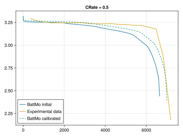
Set up the second calibration
The second calibration is performed against the 2.0C discharge curve. In the same manner as for the first discharge curve, we set up a set of parameters to calibrate against experimental data. The parameters are:
The reaction rate constant of both electrodes
The diffusion coefficient of both electrodes
The calibration this time around starts from the parameters calibrated in the first step, so we use the cell_parameters_calibrated from the first solve call when defining the new object:
t_exp_2, V_exp_2 = get_tV(df_2)

cycling_protocol2 = deepcopy(cycling_protocol)
cycling_protocol2["DRate"] = 2.0
sim2 = Simulation(model_setup, cell_parameters_calibrated, cycling_protocol2)
output2 = solve(sim2);
t2, V2 = get_tV(output2)

sim2_0 = Simulation(model_setup, cell_parameters, cycling_protocol2)
output2_0 = solve(sim2_0);
t2_0, V2_0 = get_tV(output2_0)

vc2 = VoltageCalibration(t_exp_2, V_exp_2, sim2)

free_calibration_parameter!(vc2,
    ["NegativeElectrode","ActiveMaterial", "ReactionRateConstant"];
    lower_bound = 1e-16, upper_bound = 1e-10)
free_calibration_parameter!(vc2,
    ["PositiveElectrode","ActiveMaterial", "ReactionRateConstant"];
    lower_bound = 1e-16, upper_bound = 1e-10)

free_calibration_parameter!(vc2,
    ["NegativeElectrode","ActiveMaterial", "DiffusionCoefficient"];
    lower_bound = 1e-16, upper_bound = 1e-12)
free_calibration_parameter!(vc2,
    ["PositiveElectrode","ActiveMaterial", "DiffusionCoefficient"];
    lower_bound = 1e-16, upper_bound = 1e-12)
print_calibration_overview(vc2)
✔️ Validation of CellParameters passed: No issues found.
──────────────────────────────────────────────────
✔️ Validation of CyclingProtocol passed: No issues found.
──────────────────────────────────────────────────
✔️ Validation of SimulationSettings passed: No issues found.
──────────────────────────────────────────────────
Jutul: Simulating 33 minutes, 0.0002274 nanoseconds as 44 report steps
╭────────────────┬──────────┬──────────────┬──────────╮
│ Iteration type │ Avg/step │ Avg/ministep │ Total │
│ │ 34 steps │ 35 ministeps │ (wasted) │
├────────────────┼──────────┼──────────────┼──────────┤
│ Newton │ 3.47059 │ 3.37143 │ 118 (3) │
│ Linearization │ 4.47059 │ 4.34286 │ 152 (3) │
│ Linear solver │ 3.44118 │ 3.34286 │ 117 (2) │
│ Precond apply │ 0.0 │ 0.0 │ 0 (0) │
╰────────────────┴──────────┴──────────────┴──────────╯
╭───────────────┬────────┬────────────┬──────────╮
│ Timing type │ Each │ Relative │ Total │
│ │ ms │ Percentage │ ms │
├───────────────┼────────┼────────────┼──────────┤
│ Properties │ 0.2855 │ 10.50 % │ 33.6852 │
│ Equations │ 0.5679 │ 26.92 % │ 86.3216 │
│ Assembly │ 0.0722 │ 3.42 % │ 10.9727 │
│ Linear solve │ 0.1722 │ 6.34 % │ 20.3200 │
│ Linear setup │ 0.0000 │ 0.00 % │ 0.0000 │
│ Precond apply │ 0.0000 │ 0.00 % │ 0.0000 │
│ Update │ 0.0530 │ 1.95 % │ 6.2575 │
│ Convergence │ 0.4558 │ 21.60 % │ 69.2794 │
│ Input/Output │ 0.0256 │ 0.28 % │ 0.8974 │
│ Other │ 0.7880 │ 28.99 % │ 92.9830 │
├───────────────┼────────┼────────────┼──────────┤
│ Total │ 2.7179 │ 100.00 % │ 320.7169 │
╰───────────────┴────────┴────────────┴──────────╯
✔️ Validation of CellParameters passed: No issues found.
──────────────────────────────────────────────────
✔️ Validation of CyclingProtocol passed: No issues found.
──────────────────────────────────────────────────
✔️ Validation of SimulationSettings passed: No issues found.
──────────────────────────────────────────────────
Jutul: Simulating 33 minutes, 0.0002274 nanoseconds as 44 report steps
╭────────────────┬──────────┬──────────────┬──────────╮
│ Iteration type │ Avg/step │ Avg/ministep │ Total │
│ │ 32 steps │ 33 ministeps │ (wasted) │
├────────────────┼──────────┼──────────────┼──────────┤
│ Newton │ 3.8125 │ 3.69697 │ 122 (3) │
│ Linearization │ 4.8125 │ 4.66667 │ 154 (3) │
│ Linear solver │ 3.78125 │ 3.66667 │ 121 (2) │
│ Precond apply │ 0.0 │ 0.0 │ 0 (0) │
╰────────────────┴──────────┴──────────────┴──────────╯
╭───────────────┬────────┬────────────┬──────────╮
│ Timing type │ Each │ Relative │ Total │
│ │ ms │ Percentage │ ms │
├───────────────┼────────┼────────────┼──────────┤
│ Properties │ 0.2530 │ 17.49 % │ 30.8621 │
│ Equations │ 0.5402 │ 47.14 % │ 83.1861 │
│ Assembly │ 0.0652 │ 5.69 % │ 10.0473 │
│ Linear solve │ 0.1652 │ 11.42 % │ 20.1503 │
│ Linear setup │ 0.0000 │ 0.00 % │ 0.0000 │
│ Precond apply │ 0.0000 │ 0.00 % │ 0.0000 │
│ Update │ 0.0480 │ 3.32 % │ 5.8512 │
│ Convergence │ 0.0672 │ 5.87 % │ 10.3512 │
│ Input/Output │ 0.0238 │ 0.45 % │ 0.7863 │
│ Other │ 0.1249 │ 8.63 % │ 15.2376 │
├───────────────┼────────┼────────────┼──────────┤
│ Total │ 1.4465 │ 100.00 % │ 176.4721 │
╰───────────────┴────────┴────────────┴──────────╯
NegativeElectrode: Active calibration parameters
┌─────────────────────────────────────┬───────────────┬───────────────────┐
│ Name │ Initial value │ Bounds │
├─────────────────────────────────────┼───────────────┼───────────────────┤
│ ActiveMaterial.DiffusionCoefficient │ 3.9e-14 │ 1.0e-16 - 1.0e-12 │
│ ActiveMaterial.ReactionRateConstant │ 1.764e-11 │ 1.0e-16 - 1.0e-10 │
└─────────────────────────────────────┴───────────────┴───────────────────┘
PositiveElectrode: Active calibration parameters
┌─────────────────────────────────────┬───────────────┬───────────────────┐
│ Name │ Initial value │ Bounds │
├─────────────────────────────────────┼───────────────┼───────────────────┤
│ ActiveMaterial.ReactionRateConstant │ 3.626e-11 │ 1.0e-16 - 1.0e-10 │
│ ActiveMaterial.DiffusionCoefficient │ 1.25e-15 │ 1.0e-16 - 1.0e-12 │
└─────────────────────────────────────┴───────────────┴───────────────────┘Solve the second calibration problem
cell_parameters_calibrated2, = solve(vc2);
print_calibration_overview(vc2)
Calibration: Starting calibration of 4 parameters.
It. | Objective | Proj. grad | Linesearch-its
-----------------------------------------------
0 | 6.2368e-02 | 3.8804e+01 | -
LBFGS: Resetting 'm' to number of parameters: m = 4
1 | 3.4607e-03 | 3.8803e+01 | 1
2 | 2.3931e-03 | 4.8038e-01 | 2
3 | 2.2290e-03 | 2.9616e-01 | 3
4 | 1.7002e-03 | 1.4843e-01 | 1
5 | 1.4750e-03 | 9.6600e-02 | 3
6 | 1.3955e-03 | 3.6154e-02 | 2
7 | 1.3895e-03 | 1.1852e-02 | 4
8 | 1.0776e-03 | 4.2628e-02 | 2
9 | 7.7465e-04 | 8.6295e-03 | 1
LBFGS: Line search unable to succeed in 5 iterations ...
10 | 7.7228e-04 | 5.0248e-02 | 5
LBFGS: Line search unable to succeed in 5 iterations ...
11 | 7.7086e-04 | 5.3571e-02 | 5
12 | 7.2642e-04 | 5.3810e-02 | 2
13 | 7.1447e-04 | 1.8525e-03 | 1
14 | 7.1364e-04 | 6.9386e-03 | 2
Calibration: Calibration finished in 66.012896616 seconds.
NegativeElectrode: Active calibration parameters
┌─────────────────────────────────────┬───────────────┬───────────────────┬─────────────────┬─────────┐
│ Name │ Initial value │ Bounds │ Optimized value │ Change │
├─────────────────────────────────────┼───────────────┼───────────────────┼─────────────────┼─────────┤
│ ActiveMaterial.DiffusionCoefficient │ 3.9e-14 │ 1.0e-16 - 1.0e-12 │ 1.21952e-13 │ 212.7% │
│ ActiveMaterial.ReactionRateConstant │ 1.764e-11 │ 1.0e-16 - 1.0e-10 │ 9.14306e-12 │ -48.17% │
└─────────────────────────────────────┴───────────────┴───────────────────┴─────────────────┴─────────┘
PositiveElectrode: Active calibration parameters
┌─────────────────────────────────────┬───────────────┬───────────────────┬─────────────────┬──────────┐
│ Name │ Initial value │ Bounds │ Optimized value │ Change │
├─────────────────────────────────────┼───────────────┼───────────────────┼─────────────────┼──────────┤
│ ActiveMaterial.ReactionRateConstant │ 3.626e-11 │ 1.0e-16 - 1.0e-10 │ 3.55176e-11 │ -2.05% │
│ ActiveMaterial.DiffusionCoefficient │ 1.25e-15 │ 1.0e-16 - 1.0e-12 │ 4.17914e-14 │ 3243.31% │
└─────────────────────────────────────┴───────────────┴───────────────────┴─────────────────┴──────────┘Compare the results of the second calibration against the experimental data
We can now compare the results of the calibrated model against the experimental data for the 2.0C discharge curve. We compare three simulations against the experimental data:
The initial simulation with the original parameters.
The simulation with the parameters calibrated against the 0.5C discharge curve.
The simulation with the parameters calibrated against the 0.5C and 2.0C discharge curves.
sim_c2 = Simulation(model_setup, cell_parameters_calibrated2, cycling_protocol2)
output2_c = solve(sim_c2, accept_invalid = false);

t2_c = [state[:Control][:Controller].time for state in output2_c[:states]]
V2_c = [state[:Control][:Phi][1] for state in output2_c[:states]]

fig = Figure()
ax = Axis(fig[1, 1], title = "CRate = 2.0")
lines!(ax, t2_0, V2_0, label = "BattMo.jl")
lines!(ax, t2, V2, label = "BattMo.jl (after CRate=0.5 calibration)")

lines!(ax, t_exp_2, V_exp_2, label = "Experimental data")
lines!(ax, t2_c, V2_c, label = "BattMo.jl (after CRate=0.5 + Crate=2.0 calibration)", linestyle = :dash)
axislegend(position = :lb)
fig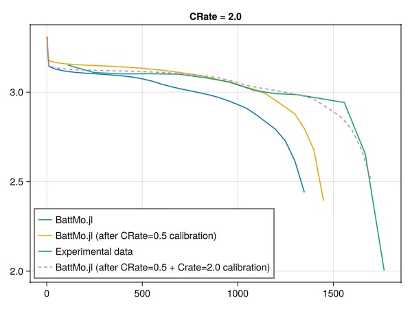
Compare the results of the calibrated model against the experimental data
We can now compare the results of the calibrated model against the experimental data for the 0.5C, 1.0C, and 2.0C discharge curves.
Note that we did not calibrate the model for the 1.0C discharge curve, but we still obtain a good fit.
CRates = [0.5, 1.0, 2.0]
outputs_base = []
outputs_calibrated = []

for CRate in CRates
	cycling_protocol["DRate"] = CRate
	simuc = Simulation(model_setup, cell_parameters, cycling_protocol)

	output = solve(simuc, info_level = -1)
	push!(outputs_base, (CRate = CRate, output = output))

    simc = Simulation(model_setup, cell_parameters_calibrated2, cycling_protocol)
	output_c = solve(simc, info_level = -1)

    push!(outputs_calibrated, (CRate = CRate, output = output_c))
end

colors = Makie.wong_colors()

fig = Figure(size = (1200, 600))
ax = Axis(fig[1, 1], ylabel = "Voltage / V", xlabel = "Time / s", title = "Discharge curve")

for (i, data) in enumerate(outputs_base)
    t_i, V_i = get_tV(data.output)
    lines!(ax, t_i, V_i, label = "Simulation (initial) $(round(data.CRate, digits = 2))", color = colors[i])
end

for (i, data) in enumerate(outputs_calibrated)
    t_i, V_i = get_tV(data.output)
	lines!(ax, t_i, V_i, label = "Simulation (calibrated) $(round(data.CRate, digits = 2))", color = colors[i], linestyle = :dash)
end

for (i, df) in enumerate(dfs)
    t_i, V_i = get_tV(df)
    label = "Experimental $(round(CRates[i], digits = 2))"
	lines!(ax, t_i, V_i, linestyle = :dot, label = label, color = colors[i])
end

fig[1, 2] = Legend(fig, ax, "C rate", framevisible = false)
fig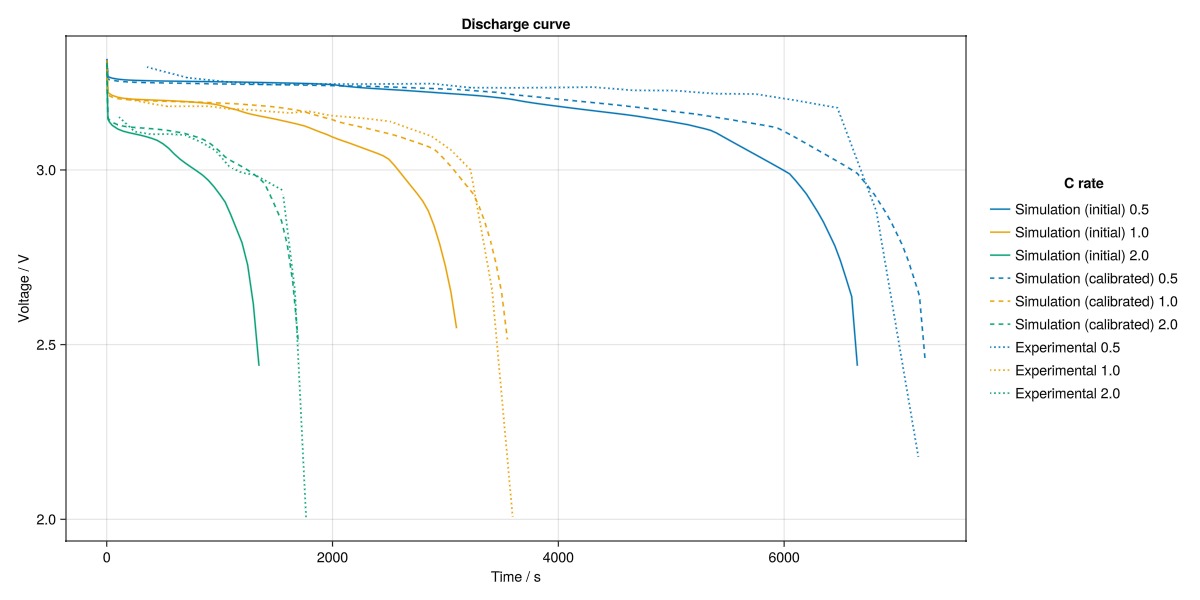
Example on GitHub
If you would like to run this example yourself, it can be downloaded from the BattMo.jl GitHub repository as a script.
This page was generated using Literate.jl.