BattMo Tutorial

Generated from battMoTutorial.m

This tutorial explains how to setup and run a simulation in BattMo

Setting up the environment

BattMo uses functionality from MRST <MRSTBattMo>. This functionality is collected into modules where each module contains code for doing specific things. To use this functionality we must add these modules to the matlab path by running:

mrstModule add ad-core mrst-gui mpfa agmg linearsolvers

Specifying the physical model

In this tutorial we will simulate a lithium-ion battery consisting of a negative electrode, a positive electrode and an electrolyte. BattMo comes with some pre-defined models which can be loaded from JSON files. Here we will load the basic lithium-ion model JSON file which comes with Battmo.

fname = fullfile('ParameterData','BatteryCellParameters',...
    'LithiumIonBatteryCell','lithium_ion_battery_nmc_graphite.json');
jsonstruct = parseBattmoJson(fname);

The parseBattmoJson function parses the JSON input and creates a matlab structure containing the same fields as the JSON input. This structure can be changed to setup the model in the way that we want. In this instance we will exclude temperature effects by setting use_thermal to false.

jsonstruct.use_thermal = false;

We will also not use current collectors in this example:

jsonstruct.include_current_collectors = false;

Our model will simulate diffusion so we set use_particle_diffusion to true:

jsonstruct.use_particle_diffusion = true;

The structure created in the jsonstruct follows the same hierarchy as the fields in the JSON input file. These can be referenced by name in the jsonstruct. To make life easier for ourselves we define some shorthand names for various parts of the structure.

ne      = 'NegativeElectrode';
pe      = 'PositiveElectrode';
elyte   = 'Electrolyte';
thermal = 'ThermalModel';
am      = 'ActiveMaterial';
itf     = 'Interface';
sd      = 'SolidDiffusion';
ctrl    = 'Control';
cc      = 'CurrentCollector';

Now we can set the diffusion model type for the active material (am) in the positive (pe) and negative (ne) electrodes to ‘full’.

jsonstruct.(pe).(am).diffusionModelType = 'full';
jsonstruct.(ne).(am).diffusionModelType = 'full';

To see which other types of diffusion model are available one can view <Electrochemistry.ActiveMaterialInputParams>. When running a simulation, BattMo requires that all model parameters are stored in an instance of BatteryInputParams. This class is used to initialize the simulation and is accessed by various parts of the simulator during the simulation. This class is instantiated using the jsonstruct we just created:

paramobj = BatteryInputParams(jsonstruct);
paramobj = paramobj.validateInputParams();

It is also possible to update the properties of this paramobj in a similar way to updating the jsonstruct. Here we set some more parameters for the diffusion model. The definitions for these are found in the corresponding classes: ActiveMaterialInputParams and FullSolidDiffusionModelInputParams.

paramobj.(ne).(am).InterDiffusionCoefficient = 0;
paramobj.(pe).(am).InterDiffusionCoefficient = 0;

paramobj.(ne).(am).(sd).N = 5;
paramobj.(pe).(am).(sd).N = 5;

Setting up the geometry

Here, we setup the 1D computational mesh that will be used for the simulation. The required discretization parameters are already included in the class BatteryGenerator1D. Classes for generating other geometries can be found in the BattMo/Battery/BatteryGeometry folder.

gen = BatteryGenerator1D();

Now, we update the paramobj with the properties of the mesh. This function will update relevent parameters in the paramobj object and make sure we have all the required parameters for the model geometry chosen.

paramobj = gen.updateBatteryInputParams(paramobj);

Initialising the battery model object

The battery model is initialized by sending paramobj to the Battery class constructor. see Battery.

model = Battery(paramobj);

In BattMo a battery model is actually a collection of submodels: Electrolyte, Negative Electrode, Positive Electrode, Thermal Model and Control Model. The battery class contains all of these submodels and various other parameters necessary to run the simulation. To see what properties the battery model object has we can print out the model variable:

model

Controlling the simulation

The control model specifies how the simulation is controlled. This can also be thought of as the boundary conditions of the simulation. In the first instance we use IEswitch control policy. (NOTE WHAT IS IESWITCH?) We set the total time scaled by the CRate in the model. The CRate has been set by the json file. We can access it here:

CRate = model.Control.CRate;
total = 1.4*hour/CRate;

We want to break this total time into 100 timesteps. To begin with we will use equal values for each timestep. We create a structure containing the length of each step in seconds (‘val’) and also which control to use for each step (‘control’). In this case we use control 1 for all steps. This means that the functions used to setup the control values are the same at each step.

n  = 100;
dt = total/n;
step = struct('val', dt*ones(n, 1), 'control', ones(n, 1));

For the IESwitch control we will switch between controlling the current or the voltage based on some max and min values. We do this using the rampupSwitchControl function. Smaller time steps are used to ramp up the current from zero to its operational value. Larger time steps are then used for the normal operation. This function also contains the logic about when to switch using constant current to constant voltage. First we set a parameter to control how the current values increase between zero and the desired value. Then we assign the rampupSwitchControl function to a variable as an anonymous function.

tup = 0.1;
srcfunc = @(time, I, E) rampupSwitchControl(time, tup, I, E, ...
                                            model.Control.Imax, ...
                                            model.Control.lowerCutoffVoltage);

We create a control structure containing the source function and specifying that we want to use IESwitch control:

control = struct('src', srcfunc, 'IEswitch', true);

Finally we collect the control and step structures together in a schedule struct which is the schedule which the simulation will follow:

schedule = struct('control', control, 'step', step);

Setting the initial state of the battery

To run simulation we need to know the starting point which we will run it from, in terms of the value of the primary variables being modelled at the start of the simulation. The initial state of the model is setup using the model.setupInitialState() method. WHAT IS HAPPENING HERE? WHAT ARE THE INITIAL VALUES SET TO?

initstate = model.setupInitialState();

Running the simulation

Once we have the initial state, the model and the schedule, we can call the simulateScheduleAD function which will actually run the simulation:

[wellSols, states, report] = simulateScheduleAD(initstate, model, schedule);

The outputs from the simulation are: - wellSols: which provides the current and voltage of the battery at each timestep. (This naming convention is a hangover from MRST where we model reservoir injection via injection wells). - states: which contains the values of the primary variables in the model at each timestep. - reports: which contains technical information about the steps used in the numerical solvers.

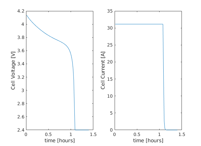
Plotting the results

To get the results we use the matlab cellfun function to extract the values Control.E, Control.I and time from each timestep (cell in the cell array) in states. We can then plot the vectors.

E = cellfun(@(x) x.Control.E, states);
I = cellfun(@(x) x.Control.I, states);
time = cellfun(@(x) x.time, states);

figure()
subplot(1,2,1)
plot(time/hour, E)
xlabel('time [hours]')
ylabel('Cell Voltage [V]')

subplot(1,2,2)
plot(time/hour, I)
xlabel('time [hours]')
ylabel('Cell Current [A]')

model =

  Battery with properties:

                           con: [1×1 PhysicalConstants]
                   Electrolyte: [1×1 Electrolyte]
             NegativeElectrode: [1×1 Electrode]
...